CMSC 455 Lecture 7, Integration

    <- previous    index    next ->

Lecture 7, Numerical Integration


Numerical Integration is usually called Numerical Quadrature.
Watch for "int" in this page it is short for "integrate".

Numerical integration could be simple summation, but
in order to get reasonable step size and good accuracy
we need better techniques.

integral f(x) dx from x=a to x=b with step size h=(b-a)/n
using simple summation would be computed:

    area = (b-a)/n * ( sum i=0..n-1  f(a+i*h) )  not using f(b)
or
    area = (b-a)/(n+1) * ( sum i=0..n  f(a+i*h) )

"h" has become the approximation to "dx" using "n" steps.
A larger value of "n" gives a smaller value of "h" and
up to where round off error grows, a better approximation.
Shown is n=9 indicated by red dots.



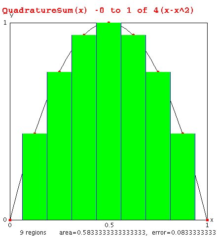from QuadratureSum.java
Exact solution integral from 0 to 1 of 4(x-x^2) = 2/3 = 0.6666666 

Trapezoidal method
The Trapezoidal rule approximates the area between x and x+h
as  h * (f(x)+f(x+h))/2 , base times average height.
Summing the areas we note that f(a) and f(b) are used once
while the other intermediate f(x) are used twice, thus:

  area = (b-a)/n * ( (f(a)+f(b))/2 + sum i=1..n-1  f(a+i*h) )

  note: i=0 is f(a)  i=n is f(b) thus sum index range 1..n-1
        h = (b-a)/n
        cutting h in half generally cuts the error in half for large n
Shown is n=8 regions based on 7 sums plus (f(a)+f(b))/2



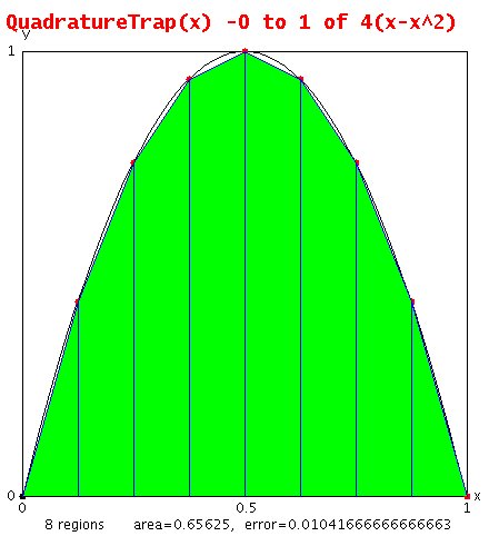from QuadratureTrap.java

trapezoide.py  Trapezoidal Integration
output is:
trapezoide.py running
trap_int area under x*x from  1.0  to  2.0  =  2.335
trapezoide.py finished
or trapezoide.py3 Trapezoidal Integration


trapezoide.java  Trapezoidal Integration
output is:
trapezoide.java running
trap_int area under x*x from 1.0 to 2.0 = 2.3350000000000004
trapezoide.java finished


You do not need to use equal step sizes.
For better accuracy with trapazoidal integration,
use smaller step size where slope is largest.
Generally this requires more steps.


Better accuracy
In order to get better accuracy with fewer evaluations of
the function, f(x), we have found a way to choose the values
of x and to apply a weight, w(x) to each evaluation of f(x).
The integral is evaluated using:

  area = sum i=1..n  w(i)*f(x(i))

The w(i) and x(i) are computed using the Legendre polynomials
covered in the previous lecture. The numerical analysis shows
that using n evaluations we obtain accuracy about equal to
fitting the f(x(i)) with an nth order polynomial and accurately
computing the integral using that nth order polynomial.

Some values of weights w(i) and ordinates x(i)  -1 < x < 1 are:

x[1]=  0.0000000000000E+00, w[1]=  2.0000000000000E+00 

x[1]= -5.7735026918963E-01, w[1]=  1.0000000000000E-00 
x[2]=  5.7735026918963E-01, w[2]=  1.0000000000000E-00 

x[1]= -7.7459666924148E-01, w[1]=  5.5555555555555E-01 
x[2]=  0.0000000000000E+00, w[2]=  8.8888888888889E-01 
x[3]=  7.7459666924148E-01, w[3]=  5.5555555555555E-01 

x[1]= -8.6113631159405E-01, w[1]=  3.4785484513745E-01 
x[2]= -3.3998104358486E-01, w[2]=  6.5214515486255E-01 
x[3]=  3.3998104358486E-01, w[3]=  6.5214515486255E-01 
x[4]=  8.6113631159405E-01, w[4]=  3.4785484513745E-01 

x[1]= -9.0617984593866E-01, w[1]=  2.3692688505618E-01 
x[2]= -5.3846931010568E-01, w[2]=  4.7862867049937E-01 
x[3]=  0.0000000000000E+00, w[3]=  5.6888888888889E-01 
x[4]=  5.3846931010568E-01, w[4]=  4.7862867049937E-01 
x[5]=  9.0617984593866E-01, w[5]=  2.3692688505618E-01 

x[1]= -9.3246951420315E-01, w[1]=  1.7132449237916E-01 
x[2]= -6.6120938646626E-01, w[2]=  3.6076157304814E-01 
x[3]= -2.3861918608320E-01, w[3]=  4.6791393457269E-01 
x[4]=  2.3861918608320E-01, w[4]=  4.6791393457269E-01 
x[5]=  6.6120938646626E-01, w[5]=  3.6076157304814E-01 
x[6]=  9.3246951420315E-01, w[6]=  1.7132449237916E-01 

For a range from a to b, new_x[i] = a+(x[i]+1)*(b-a)/2



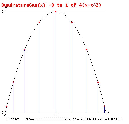from QuadratureGau.java
and  gauleg.java


Using the function  gaulegf  a typical integration could be:

  double x[9], w[9]     for 8 points
  a = 0.5;  integrate sin(x) from a to b
  b = 1.0;
  n = 8;
  gaulegf(a, b, x, w, n);   x's adjusted for a and b
  area = 0.0;
  for(j=1; j<=n; j++)
      area = area + w[j]*sin(x[j]);


The following programs, gauleg for Gauss Legendre integration,
computes the x(i) and w(i) for various values of n. The
integration is tested on a constant f(x)=1.0 and then on
integral sin(x) from x=0.5 to x=1.0
integral exp(x) from x=0.5 to x=5.0
integral ((x^x)^x)*(x*(log(x)+1)+x*log(x)) from x=0.5 to x=5.0
         This is labeled "mess" in output files.

Note how the accuracy increases with increasing values of n,
then, no further accuracy is accomplished with larger n.

Also note, the n where best numerical accuracy is achieved
is a far smaller n than where round off error would be
significant.


Downloadable code in C, Python, Fortran, Java, Ada and Matlab
Choose your favorite language and study the .out file
then look over the source code.

Just testing gaulegf:

integrate3d.java calculus
integrate3d_java.out numerical

gauleg.py  function is gaulegf
test_gauleg.py
test_gauleg_py.out
gauleg.py3  function is gaulegf
test_gauleg.py3
test_gauleg_py3.out

gaulegf.java
test_gauleg.java
test_gauleg_java.out

gaulegf.h
gaulegf.c
test_gaulegf.c
test_gaulegf_c.out

test_gaulegf.cpp C++
test_gaulegf_cpp.out result

test_gaulegf.rb Ruby
test_gaulegf_rb.out result

gaulegf.adb
test_gaulegf.adb
test_gaulegf_ada.out

gaulegf.f90 original


Look near end of  .out  file, note convergence to exact value at end.
integral sin(x) from x=0.5 to x=1.0  for order 2 through 10
integral exp(x) from x=0.5 to x=5.0  for order 2 through 10
integral ((x^x)^x)*(x*(log(x)+1)+x*log(x)) from x=0.5 to x=5.0
         This is labeled "mess" in output files. order 2 through 30



gauleg.c
gauleg_c.out

gauleg.f90
gauleg_f90.out

gauleg.for
gauleg_for.out

gauleg.java
gauleg_java.out

gauleg.adb
gauleg_ada.out

gaulegf.m
gauleg.m
gauleg_m.out

On Linux, you may use  octave  rather than  MatLab.

Higher dimension, more independent variables
Multidimensional integration extends easily by using

  gaulegf(ax, bx, xx, wx, nx);   x's adjusted for ax and bx
  gaulegf(ay, by, yy, wy, ny);   y's adjusted for ay and by
  volume = 0.0;
  for(i=1; i<=nx; i++)
    for(j=1; j<=ny; j++)
      volume = volume + wx[i]*wy[j]*f(xx[i],yy[j]);


  gaulegf(ax, bx, xx, wx, nx);   x's adjusted for ax and bx
  gaulegf(ay, by, yy, wy, ny);   y's adjusted for ay and by
  gaulegf(az, bz, zz, wz, nz);   z's adjusted for az and bz
  volume4d = 0.0;
  for(i=1; i<=nx; i++)
    for(j=1; j<=ny; j++)
      for(k=1; k<=nz; k++)
        volume4d = volume4d + wx[i]*wy[j]*wz[k]*f(xx[i],yy[j],zz[k]);

Volume code as shown in:

int2d.c
int2d_c.out


Additional reference books include:

"Handbook of Mathematical Functions" by Abramowitz and Stegun
A classic reference book on numerical integration and differentiation.

"Numerical Recipes in Fortran" by Press, Teukolsky, Vetterling and Flannery
There is also a "Numerical recipes in C" yet in my copy, there have
been a number of errors in the C code due to poor translation from Fortran.
Many very good numerical codes for general purpose and special purposes.

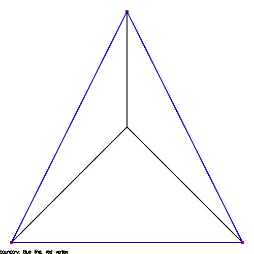
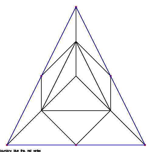
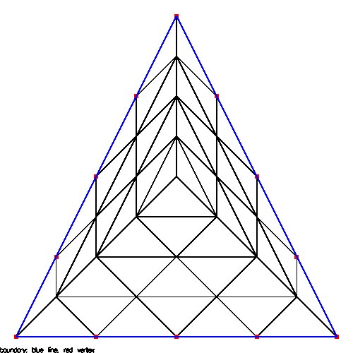
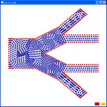
Integration of functions over triangles
An impressive example of quadrature over triangles is shown
by using Gauss Legendre integration coordinates rather than
splitting a triangle into smaller congruent triangles.
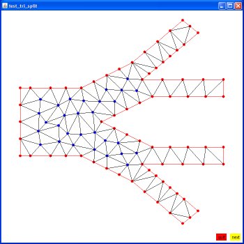
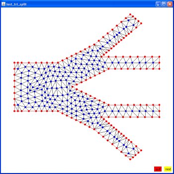
The routine "tri_split" converts a single triangle into four
congruent triangles that exactly cover the initial triangle.
Linear quadrature then uses just the center point of the
split, four equal area, triangles.
triquad.java triangle quadrature
test_triquad.java test
test_triquad.out results, see last two sets

Reducing the step size improves integration accuracy.
In two or more dimensions, reducing area, volume, etc.
improves integration accuracy. Two sets of triangle
splitting are shown below. Using higher order integration
provides more integration accuracy than smaller step size,
smaller area, volume, etc.

From tri_split.java
and  test_tri_split.java










These will appear later in the solution of
partial differential equations using the Finite Element Method.

determine if a point is inside a polygon
point_in_poly.c
point_in_poly_c.out
point_in_poly.java
point_in_poly_java.out


Digitizing curves into computer
Scan the curve you want to digitize, sample curves listed below.
Compile Digitize.java
Run  java Digitize your.jpg > your.out
Edit your.out to suit your needs. Output is scaled to your first 3 points.
(0,0) (1,0) (0,1)
Additional binary graphics files are:
pi.gif
curve.jpg
c6thrust.jpg
chess2.png
Digitize.out some output from curve.jpg


When working with calculus, you may encounter the "divergence theorem"
For a vector function F in a volume V with surface S
integrate over volume (∇˙F)dV = 
integrate over surface (F˙normal)dS



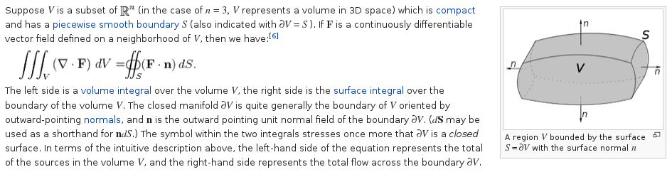Just for fun, I programmed a numerical test to check the theorem
for one specific case:  program and results of run
divergence_theorem.c
divergence_theorem_c.out

 The general form of the trapezoidal integration.
a = integral y(x) dx over a set of increasing values of x, x_1 to x_n, 
a = sum i=1 to i=n-1 of (x_i+1 - x_i) * (y(x_i) + y(x_i+1))/2
The (x_i+1 - x_i) is a variable version of h.
For best accuracy, pick x values where slope is changing,
in general use  dx  smaller for larger slope. 

HW3 is assigned