<- previous index next ->
A function may be given as an analytic expression
such as sqrt(exp(x)-1.0) or may be given as a set
of points (x_i, y_i).
There are occasions when an efficient and convenient computer
implementation is needed. One of the efficient and convenient
implementations is a polynomial.
Thanks to Mr. Taylor and Mr. Maclaurin we can convert any
continuously differentiable function to a polynomial:
Taylor series, given differentiable function, f(x)
pick a convenient value for a
(x-a) f'(a) (x-a)^2 f''(a) (x-a)^3 f'''(a)
f(x) = f(a) + ----------- + -------------- + --------------- + ...
1! 2! 3!
Maclaurin series, same as Taylor series with a=0
x f'(0) x^2 f''(0) x^3 f'''(0)
f(x) = f(0) + ------- + ---------- + ----------- + ...
1! 2! 3!
Taylor series, function offset by value of h
h f'(x) h^2 f''(x) h^3 f'''(x)
f(x+h) = f(x) + ------- + ---------- + ----------- + ...
1! 2! 3!
Please use analytic differentiation rather than numerical differentiation.
Programs such as Maple have Taylor Series generation as a primitive.
An example Taylor series is: e^x = 1 + x + x^2/2! + x^3/3! + x^4/4!
Using a fixed number of terms, fourth power in this example,
will result in truncation error. The series has been truncated.
It should be obvious, that for large x, the error will become
very large. Also, this type of series will fail or be very
inaccurate if there are discontinuities in the function being fit.
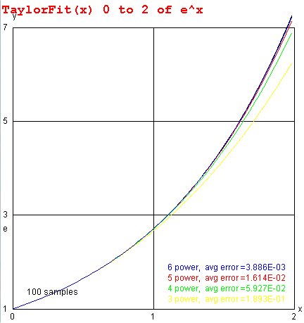
We often estimate "truncation" error as the next order term
that is not used.
Note the relation of "estimated truncation error" to maximum error
and rms error as more terms are used in the approximation.
TaylorFit.java
TaylorFit_java.out
It is interesting to note that: The truncation error is usually
slightly less than the maximum error, thus a reasonable estimate
of the accuracy of the fit.
Unequally spaced points often use least square fit
For functions given as unequally spaced points, use
the least square fit technique in Lecture 4
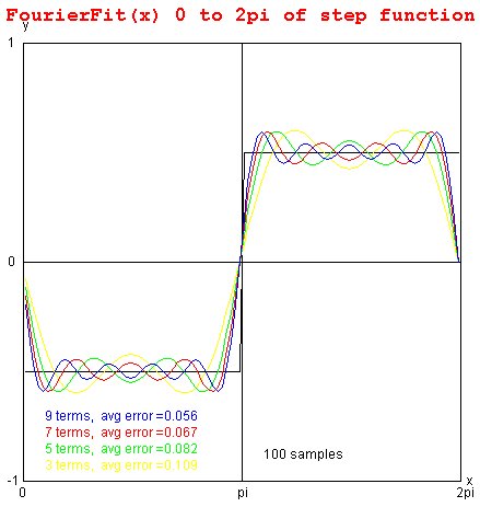
Fitting discontinuous data, try Fourier Series
For function with discontinuities the Fourier Series or
Fejer Series may produce the required fit.
The Fourier series approximation f(t) to f(x) is defined as:
f(t) = a_0/2 + sum n=1..N a_n cos(n t) + b_n sin(n t)
a_n = 1/Pi integral -Pi to Pi f(x) cos(n x) dx
b_n = 1/Pi integral -Pi to Pi f(x) sin(n x) dx
When given an analytic function, f(x) it may be best to use analytic
evaluation of the integrals. When given just points it may be best
to not use Fourier series, use Lagrange fit.
 FourierFit.java
FourierFit.out
test_fourier.java source code
test_fourier_java.out output
test_fourier.dat for ploting
FourierFit.java
FourierFit.out
test_fourier.java source code
test_fourier_java.out output
test_fourier.dat for ploting
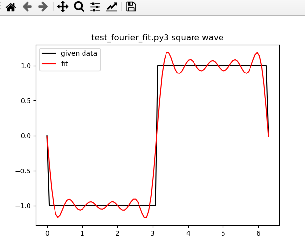 test_fourier_fit.py3
test_fourier_fit_py3.out
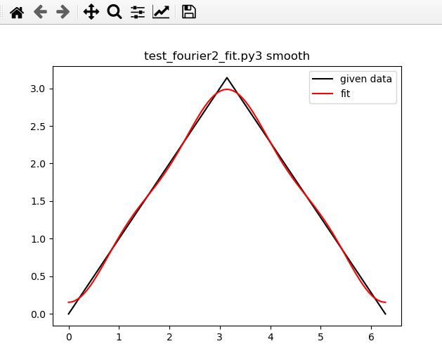
test_fourier_fit.py3
test_fourier_fit_py3.out
 test_fourier_fit.py3
test_fourier_fit_py3.out
test_fourier_fit.py3
test_fourier_fit_py3.out
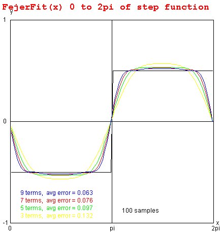
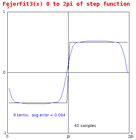
Smoothing discontinuous data with Fejer Series
The Fejer series approximation f(t) to f(x) is defined as:
f(t) = a_0/2 + sum n=1..N a_n (N-n+1)/N cos(n t) + b_n (N-n+1)/N sin(n t)
a_n = 1/Pi integral -Pi to Pi f(x) cos(n x) dx
b_n = 1/Pi integral -Pi to Pi f(x) sin(n x) dx
Basically the Fejer Series with the contribution of the higher
frequencies increased. This will give a smoother fit
with less oscillations. See plot for square wave.
 FejerFit.java
FejerFit.out
test_fejer.java source code
test_fejer_java.out output
test_fejer.dat for ploting
FejerFit.java
FejerFit.out
test_fejer.java source code
test_fejer_java.out output
test_fejer.dat for ploting
 FejerFit3.java
FejerFit3_java.out
FejerFit3.java
FejerFit3_java.out
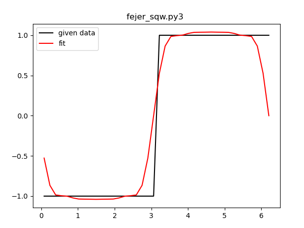 fejer_sqw.py3
fejer_sqw_py3.out
fejer_sqw.py3
fejer_sqw_py3.out
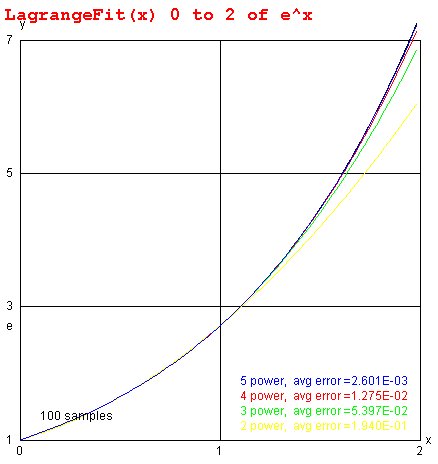
Lagrange Fit minimizes maximum error (at fit points)
The Lagrange Fit minimizes the error at the chosen points to fit.
The Lagrange Fit is good for fitting data given at uniform spacing.
The Lagrange fit requires the fewest evaluations of the function
to be fit, convenient if the function to be fit requires
significant computation time.
The Lagrange series approximation f(t) to f(x) is defined as:
L_n(x) = sum j=0..N f(x_j) L_n,j(x)
L_n,j(x) = product i=0..N i /= j (x - x_i)/(x_j - x_i)
Collect coefficients, a_n, of L_n(x) to get
f(t) = sum i=0..N a_n t^n
 LagrangeFit.java
LagrangeFit.out
LagrangeFit.java
LagrangeFit.out
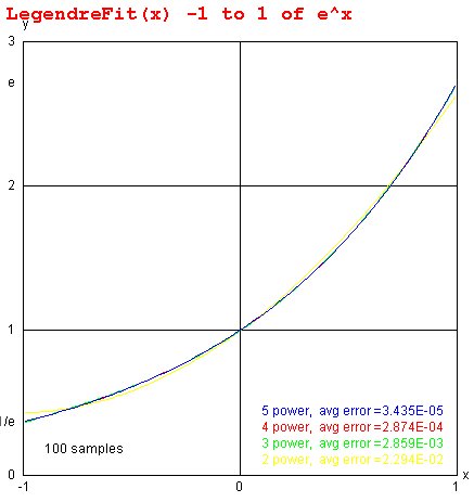
Legendre Fit minimizes RMS error
The Legendre Fit, similar to the Least Square Fit, minimizes
the RMS error of the fit.
The Legendre series approximation f(t) to f(x) is defined as:
f(t) = a_0 g_0 + sum n=1..N a_n g_n P_n(t) then combining coefficients can be
f(t) = sum n=0..n b_n t^n a simple polynomial
a_n = integral -1 to 1 f(x) P_n(x) dx
g_n = (2 n + 1)/2
P_0(x) = 1
P_1(x) = x
P_n(x) = (2n-1)/n x P_n-1(x) - (n-1)/n P_n-2(x)
Suppose f(x) is defined over the interval a to b, rather than -1 to 1, then
a_n = (b-a)/2 integral -1 to 1 f(a+b+x(b-a)/2) P_n(x) dx
 LegendreFit.java
LegendreFit.out
LegendreFit.java
LegendreFit.out
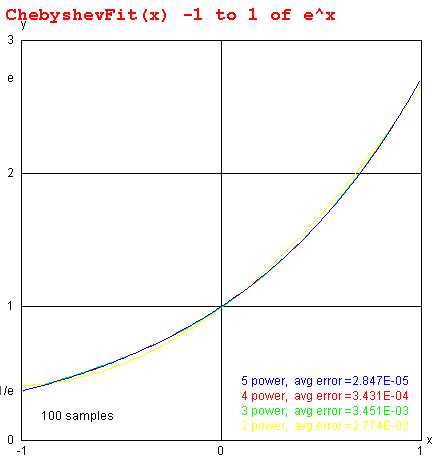
Chebyshev Fit minimizes maximum error (at fit points)
The Chebyshev Fit minimizes to maximum error of the fit for
a given order polynomial.
The Chebyshev series approximation f(t) to f(x) is defined as:
f(t) = a_0/2 + sum n=1..N a_n T_n(t) then combining coefficients can be
f(t) = sum n=0..n b_n t^n a simple polynomial
a_n = 2/Pi integral -1 to 1 f(x) T_n(x)/sqrt(1-x^2) dx
T_0(x) = 1
T_1(x) = x
T_n+1(x) = 2 x T_n(x) - T_n-1(x)
for -1 < x < 1 T_n(x) = cos(n acos(x))
When given an analytic function it may be best to use analytic
evaluation of the integrals. When given just points it may be best
to not use Chebyshev fit, use Lagrange fit. When given a
computer implementation of the function, f(x), to be fit,
use a very good adaptive integration.
 ChebyshevFit.java
ChebyshevFit.out
Note good intermediate points on smoth curve.
ChebyshevFit.java
ChebyshevFit.out
Note good intermediate points on smoth curve.
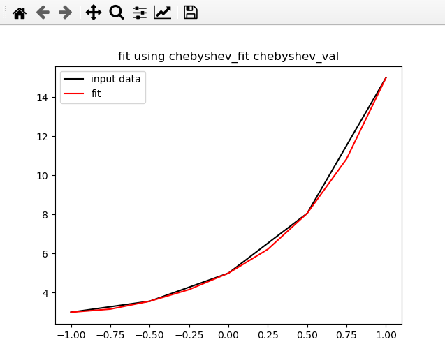 test_chebyshev_fit.py3
test_chebyshev_fit_py3.out
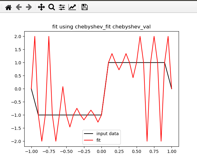
Note bad intermediate points on square wave.
test_chebyshev_fit.py3
test_chebyshev_fit_py3.out
Note bad intermediate points on square wave.
 chebyshev_sqw.py3
Chebyshev_sqw_py3.out
chebyshev_sqw.py3
Chebyshev_sqw_py3.out
spline fit exact at data points with approximate slope
Involves computing derivatives and solving simultaneous equations
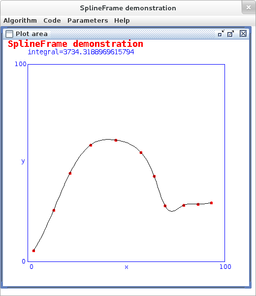 Spline.java
Spline.out
SplineFrame.java
SplineFrame.out
SplineHelp.txt
SplineAbout.txt
SplineAlgorithm.txt
SplineIntegrate.txt
SplineEvaluate.txt
Source code and text output for the various fits:
LagrangeFit.java
LagrangeFit.out
LegendreFit.java
LegendreFit.out
FourierFit.java
FourierFit.out
FejerFit.java
FejerFit.out
ChebyshevFit.java
ChebyshevFit.out
You may convert any of these that you need to a language
of your choice.
learn language to convert to or from
Spline.java
Spline.out
SplineFrame.java
SplineFrame.out
SplineHelp.txt
SplineAbout.txt
SplineAlgorithm.txt
SplineIntegrate.txt
SplineEvaluate.txt
Source code and text output for the various fits:
LagrangeFit.java
LagrangeFit.out
LegendreFit.java
LegendreFit.out
FourierFit.java
FourierFit.out
FejerFit.java
FejerFit.out
ChebyshevFit.java
ChebyshevFit.out
You may convert any of these that you need to a language
of your choice.
learn language to convert to or from
Interactive Demonstration
Examples of interactive fitting of points may run:
java -cp . LeastSquareFitFrame
java -cp . LagrangeFitFrame
java -cp . SplineFrame
Lagrange.java
TestLagrange.java
TestLagrange.out
LagrangeFitFrame.java
LagrangeHelp.txt
LagrangeAbout.txt
LagrangeAlgorithm.txt
LagrangeIntegrate.txt
LagrangeEvaluate.txt
LeastSquareFit.java
LeastSquareFitFrame.java
LeastSquareFitHelp.txt
LeastSquareFitAbout.txt
LeastSquareFitAlgorithm.txt
LeastSquareFitIntegrate.txt
LeastSquareFitEvaluate.txt
<- previous index next ->
-
CMSC 455 home page
-
Syllabus - class dates and subjects, homework dates, reading assignments
-
Homework assignments - the details
-
Projects -
-
Partial Lecture Notes, one per WEB page
-
Partial Lecture Notes, one big page for printing
-
Downloadable samples, source and executables
-
Some brief notes on Matlab
-
Some brief notes on Python
-
Some brief notes on Fortran 95
-
Some brief notes on Ada 95
-
An Ada math library (gnatmath95)
-
Finite difference approximations for derivatives
-
MATLAB examples, some ODE, some PDE
-
parallel threads examples
-
Reference pages on Taylor series, identities,
coordinate systems, differential operators
-
selected news related to numerical computation