<- previous index next ->
A polynomial of degree n has the largest exponent value n.
There are n+1 terms and n+1 coefficients.
A normalized polynomial has the coefficient of the
largest exponent equal to 1.0.
An nth order polynomial with coefficients c_0 through c_n.
y = c_0 + c_1 x + c_2 x^2 +...+ c_n-1 x^n-1 + c_n x^n
Horners method for evaluating a polynomial
"y" is computed numerically using Horners method that
needs n multiplications and n additions.
Thus faster and more accurate.
Starting at the highest power, set y = c_n * x
Then combine the next coefficient y = (c_n-1 + y) * x
Continue for c_n-2 until c_1 y = (c_1 + y) * x
Then finish y = c_0 + y
The code in C, Fortran 90, Java and Ada 95 is:
/* peval.c Horners method for evaluating a polynomial */
double peval(int n, double x, double c[])
{ /* an nth order polynomial has n+1 coefficients */
/* stored in c[0] through c[n] */
/* y = c[0] + c[1]*x + c[2]*x^2 +...+ c[n]*x^n */
int i;
double y = c[n]*x;
if(n<=0) return c[0];
for(i=n-1; i>0; i--) y = (c[i]+y)*x;
return y+c[0];
} /* end peval */
! peval.f90 Horners method for evaluating a polynomial
function peval(n, x, c) result (y)
! an nth order polynomial has n+1 coefficients
! stored in c(0) through c(n)
! y = c(0) + c(1)*x + c(2)*x^2 +...+ c(n)*x^n
implicit none
integer, intent(in) :: n
double precision, intent(in) :: x
double precision, dimension(0:n), intent(in) :: c
double precision :: y
integer i
if(n<=0) y=c(0); return
y = c(n)*x
do i=n-1, 1, -1
y = (c(i)+y)*x
end do
y = y+c(0)
end function peval
// peval.java Horners method for evaluating a polynomial
double peval(int n, double x, double c[])
{ // an nth order polynomial has n+1 coefficients
// stored in c[0] through c[n]
// y = c[0] + c[1]*x + c[2]*x^2 +...+ c[n]*x^n
double y = c[n]*x;
if(n<=0) return c[0];
for(int i=n-1; i>0; i--) y = (c[i]+y)*x;
return y+c[0];
} // end peval
-- peval.adb Horners method for evaluating a polynomial
function peval(n : integer; x : long_float; c : vector) return long_float is
-- an nth order polynomial has n+1 coefficients
-- stored in c(0) through c(n)
-- y := c(0) + c(1)*x + c(2)*x^2 +...+ c(n)*x^n
y : long_float;
begin
if n<=0 then return c(0); end if;
y := c(n)*x;
for i in reverse 1..n-1 loop -- do i:=n-1, 1, -1
y := (c(i)+y)*x;
end loop;
y := y+c(0);
return y;
end peval;
MatLab
y = polyval(c, x)
Python
from numpy import polyval
y = polyval(c, x)
Testing high degree polynomials
Although Horners method is fast and accurate on most polynomials,
the following test programs in C, Fortran 90, Java and Ada95
show that evaluating polynomials of order 9 and 10 can have
significant absolute error.
The test programs generate a set of roots r_0, r_1, ...
and computer the coefficients of a set of polynomials
y = (x-r_0)*(x-r_1)*...*(x-r_n-1) becomes
y = c_0 + c_1*x + c_2*x^2 +...+ c_n-1*x^n-1 + 1.0*x^n
when x is any of the roots, y should be zero.
Study one of the .out files and see how the absolute
error increases with polynomial degree and increases with
the magnitude of the root.
(The source code was run on various types of computers
and various operating systems. Results vary.)
peval.c
peval_c.out
peval.f90
peval_f90.out
peval.java
peval_java.out
peval.adb
peval_ada.out
test_peval.rb
test_peval_rb.out
Having the coefficients of a polynomial allows creating
the derivative and integral of the polynomial.
Derivative of Polynomial
Given:
y = c_0 + c_1 x + c_2 x^2 +...+ c_n-1 x^n-1 + c_n x^n
dy/dx = c_1 + 2 c_2 x + 3 c_3 x^2 +...+ n-1 c_n-1 x^n-2 + n c_n x^n-1
The coefficients of dy/dx may be called cd and computed:
for(i=0; i<n; i++) cd[i] = (double)(i+1)*c[i+1];
nd = n-1;
The derivative may be computed an any point, example x=a, using
dy_dx_at_a = peval(nd, a, cd);
Integral of Polynomial
Similarly, the integral y(x) dx has coefficients
Given:
y = c_0 + c_1 x + c_2 x^2 +...+ c_n-1 x^n-1 + c_n x^n
int_y_dx = 0 + c_0 x + c_1/2 x^2 +...+ c_n-1/n x^n + c_n/(n+1) x^n+1
The coefficients of int_y_dy may be called ci and computed:
ci[0] = 0.0; /* a reasonable choice */
ni = n+1;
for(i=1; i<=ni; i++) ci[i] = c[i-1]/(double)i;
The integral of the original polynomial y from a to b is computed:
int_y_a_b = peval(ni, b, ci) - peval(ni, a, ci);
Polynomial Arithmetic
The sum, difference, product and quotient of two polynomials p and q are:
(unused locations filled with zeros)
nsum = max(np,nq);
for(i=0; i<=nsum; i++) sum[i] = p[i] + q[i];
ndifference = max(np,nq);
for(i=0; i<=ndifference; i++) difference[i] = p[i] - q[i];
nproduct = np+nq;
for(i=0; i<=nproduct; i++) product[i] = 0.0;
for(i=0; i<=np; i++)
for(j=0; j<=nq; j++) product[i+j] += p[i]*q[j];
/* np > nd */
nquotient = np-nd;
nremainder = np
k = np;
for(j=0; j<=np; j++) r[j] = p[j]; /* initial remainder */
for(i=nquotient; i>=0; i--)
{
quotient[i] = r[k]/d[nd]
for(j=nd; j>=0; j--) r[k-nd+j] = r[k-nd+j] - quotient[i]*d[j]
k--;
}
Polynomial operations including add,sub,mul,div,roots,deriv,integral
poly.h
poly.c
test_poly.c
test_poly_c.out
poly.java
test_poly.java
test_poly_java.out
In Python all available import numpy.matlib
To see all functions print dir(numpy.matlib)
Polynomial series
Taylor series, for any differentiable function, f(x)
(x-a) f'(a) (x-a)^2 f''(a) (x-a)^3 f'''(a)
f(x) = f(a) + ----------- + -------------- + --------------- + ...
1! 2! 3!
MacLaurin series, Taylor series with a=0
x f'(0) x^2 f''(0) x^3 f'''(0)
f(x) = f(0) + ------- + ---------- + ----------- + ...
1! 2! 3!
Taylor series, offset
h f'(x) h^2 f''(x) h^3 f'''(x)
f(x+h) = f(x) + ------- + ---------- + ----------- + ...
1! 2! 3!
Example f(x) = e^x, thus f'(x) = e^x f''(x) = e^x f'''(x) = e^x
f(0) = 1 f'(0) = 1 f''(0) = 1 f'''(0) = 1
substituting in the MacLaurin series
x x^2 x^3 x^4
f(x) = 1 + -- + --- + --- + --- + ...
1! 2! 3! 4!
Example f(x) = sin(x), f'(x) = cos(x) f''(x) = -sin(x) f'''(x) = -cos(x)
f(0) = 0 f'(0) = 1 f''(0) = 0 f'''(0) = -1
substituting in the MacLaurin series
x x^3 x^5 x^7
f(x) = -- - --- + --- - --- + ...
1! 3! 5! 7!
Example f(x) = cos(x), f'(x) = -sin(x) f''(x) = -cos(x) f'''(x) = sin(x)
f(0) = 1 f'(0) = 0 f''(0) = -1 f'''(0) = 0
substituting in the MacLaurin series
x^2 x^4 x^6
f(x) = 1 - --- + --- - --- + ...
2! 4! 6!
Many MacLaurin series expansions are shown on Mathworld
Taylor and MacLaurin series can be expanded for two and more variables.
Two dimensional Taylor series expansion is here
Orthogonal Polynomials
For use in integration and fitting data by a polynomial,
orthogonal polynomials are used. The definition of orthogonal
is based on having a set of polynomials from degree 0 to
degree n that are denoted by p_0(x), p_1(x),...,p_n-1(x), p_n(n).
A weighting function is allowed, w(x), that depends on x but
not on the degree of the polynomial. The set of polynomials
is defined as orthogonal over the interval x=a to x=b when
the following two conditions are satisfied:
/ 0 if i != j
integral from x=a to x=b of w(x) p_i(x) p_j(x) dx = |
\ not 0 if i=j
sum from i=1 to i=n c_i *p_i(x) = 0 for all x only when all c_i are zero.
Legendre Polynomials, Chebyshev Polynomials, Laguerre Polynomials and
Lagrange Polynomials are covered below.
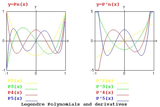
Legendre Polynomials
P_n(x) are defined as
P_0(x) = 1
P_1(x) = x
P_2(x) = 1/2 (3 x^2 - 1)
P_3(x) = 1/2 (5 x^3 - 3 x)
P_4(x) = 1/8 (35 x^4 - 30 x^2 + 3)
the general recursion formula for P_n(x) is
P_n(x) = 2n-1/n x P_n-1(x) - n-1/n P_n-2(x)
The weight function is w(x) = 1
The interval is a = -1 to b = 1
Explicit expression
P_n(x) = 1/2^n sum m=0 to n/2
(-1)^m (2n-2m)! / [(n-m)! m! (n-2m)!] x^(n-2m)
P_n(x) = (-1)^n/(2^n n!) d^n/dx^n ((1-x^2)^n)
Legendre polynomials are best known for use in Gaussian
integration. These approximate a least square fit.
integrate f(x) for x= -1 to 1
For n point integration, determine w_i and x_i i=1,n
where x_i is the i th root of P_n(x) and
w_i = (x_i)
integral x=-1 to 1 of f(x) = sum i=1 to n of w_i f(x_i)
Change interval from t in [a, b] to x in [-1, 1]
x = (b+a+(b-a)t)/2
see example test program gauleg.c
and results gauleg_c.out
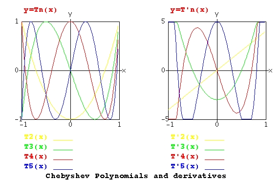
Chebyshev polynomials
T_n(x) are defined as
T_0(x) = 1
T_1(x) = x
T_2(x) = 2 x^2 - 1
T_3(x) = 4 x^3 - 3 x
T_4(x) = 8 x^4 - 8 x^2 + 1
the general recursion formula for T_n(x) is
T_n(x) = 2 x T_n-1(x) - T_n-2(x)
The weight function, w(x) = 1/sqrt(1-x^2)
The interval is a = -1 to b = 1
Explicit expression
T_n(x) = n/2 sum m=0 to n/2 (-1)^m (n-m-1)!/(m! (n-2m)!) (2x)^(n-2m)
T_n(x) = cos(n arccos(x))
Chebyshev polynomials are best known for approximating a function
while minimizing the maximum error, covered in a latter lecture.
Fit f(x) with approximate function F(x)
c_i = 2/pi integral x=-1 to 1 f(x) T_i(x) /sqrt(1-x^2) dx
(difficult near x=-1 and x=1)
F(x) = c_0 /2 + sum i=1 to n c_i T_i(x)
Change interval from t in [a, b] to x in [-1, 1]
x = (b+a+(b-a)t)/2
see example test program chebyshev.c
and results chebyshev_c.out
Laguerre polynomials
L_n(x) are defined as
L_0(x) = 1
L_1(x) = -x + 1
L_2(x) = x^2 - 4 x + 2
L_3(x) = -x^3 +9 x^2 - 18 x + 6
the general recursion formula for L_n(x) is
L_n(x) = (2n-x-1) L_n-1(x) - (n-1)^2 L_n-2(x)
The weight function, w(x) = e^(-x)
The interval is a = 0 to b = infinity
Explicit expression
L_n(x) = sum m=0 to n (-1)^m n!/(m! m! (n-m)!) x^m
L_n(x) = 1/(n! e^-x) d^n/dx^n (x^n e^(-x))
Laguerre polynomials are best known for use in integrating
functions where the upper limit is infinity.
Lagrange Polynomials
These will be used later in Galerkin Finite Element Method
for solving partial differential equations.
Lagrange polynomials L_n(x) are defined as
L_1,0(x) = 1 - x
L_1,1(x) = x
L_2,0(x) = 1 -3 x +2 x^2
L_2,1(x) = 4 x -4 x^2
L_2,2(x) = - x +2 x^2
L_3,0(x) = 1 -5.5 x +9 x^2 -4.5 x^3
L_3,1(x) = 9 x -22.5 x^2 +13.5 x^3
L_3,2(x) = -4.5 x +18 x^2 -13.5 x^3
L_3,3(x) = x -4.5 x^2 +4.5 x^3
L_4,1(x) = 16 x -69.33 x^2 + 96 x^3 - 42.33 x^4
L_5,2(x) = -25 x +222.92 x^2 -614.58 x^3 +677.08 x^4 -260.42 x^5
For 0 ≤ x ≤ 1 and equal spaced points in between.
The general recursion formula for L_n+1,j(x) is
unavailable
Explicit expression
L_n,k(x) = product i=0 to n, i/=k of (x-x_i)/(x_k-x_i)
Lagrange polynomials are best known for solving differential
equations with equal and unequal grid spacing.
An nth order Lagrange polynomial will exactly fit n data points.
Fit f(x) with approximate function F(x)
F(x) = sum k=0 to n of f(x_k) L_n,k(x)
Change of coordinates for integration
Change interval from t in [a, b] to x in [0, 1]
x = (t-a)/(b-a)
Change interval from t in [a, b] to x in [-1, 1]
x = 2(t-a)/(b-a)-1
Example plots
see example test program lagrange.c
and results lagrange_c.out
A family of Lagrange Polynomials can be constructed to be
1.0 at x_i and zero at every x_j where i ≠ j
Using the notation above, np=11 and each color is a different k.
Each of the 11 points has one color at 1.0 and all other
colors at 0.0 .
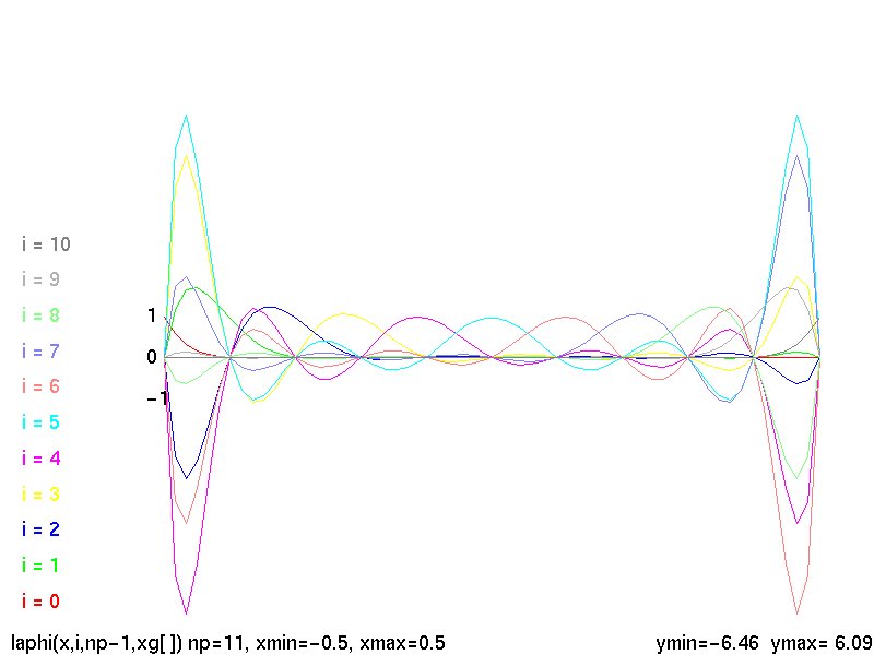 Lagrange Phi shape functions
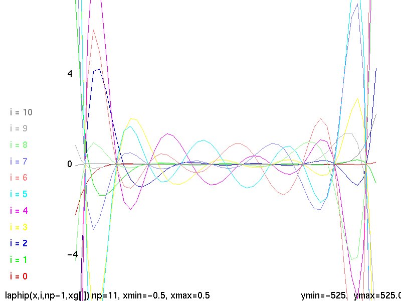 First derivative of Lagrange Phi shape functions
polynomial functions in python3
test_poly.py3 source code of functions
test_poly_py3.out output
test_poly2.py3 source code of functions
test_poly2_py3.out output
python3 divide integers produces floating point
test.py3 source code of functions
test_py3.out output
Additional utility functions:
cs455_l37.html
<- previous index next ->
-
CMSC 455 home page
-
Syllabus - class dates and subjects, homework dates, reading assignments
-
Homework assignments - the details
-
Projects -
-
Partial Lecture Notes, one per WEB page
-
Partial Lecture Notes, one big page for printing
-
Downloadable samples, source and executables
-
Some brief notes on Matlab
-
Some brief notes on Python
-
Some brief notes on Fortran 95
-
Some brief notes on Ada 95
-
An Ada math library (gnatmath95)
-
Finite difference approximations for derivatives
-
MATLAB examples, some ODE, some PDE
-
parallel threads examples
-
Reference pages on Taylor series, identities,
coordinate systems, differential operators
-
selected news related to numerical computation