<- previous index next ->
When all else fails, there is adaptive numerical quadrature.
This is cleaver because the integration adjusts to the function
being integrated. And, yes, it can have problems.
The basic principle is to divide up the integration into
intervals. Use two methods of integration in each interval.
If the two methods do not agree in some interval, divide that
interval in half, and repeat. The total integral is the sum
of the integrals of all the intervals.
Consider integrating the function y = 1/x from 0.01 to 2.0,
with a high point at y=100 with a very steep slope and
a low relatively flat area from y=1.0 to y=0.5.
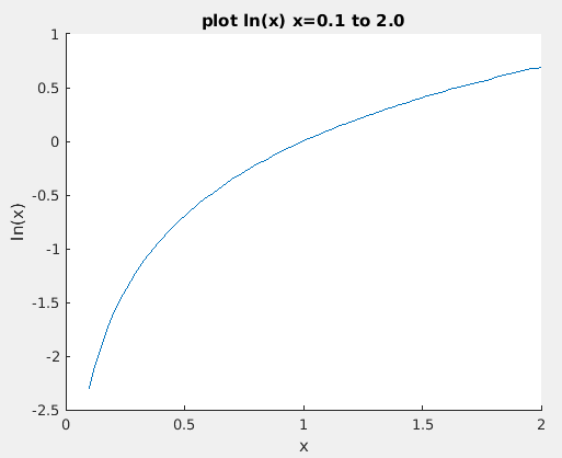
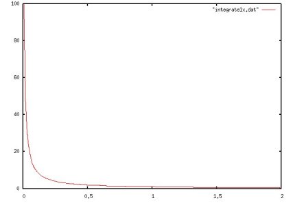 Note that the analytic solution is ln(2.0)-ln(0.01).
Do not try integration from 0 to 2, the integral is infinite.
The integral from 0.1 to 1 of 1/x = 2.302585093
The integral from 0.01 to 0.1 of 1/x = 2.302585093
The integral from 0.001 to 0.01 of 1/x = 2.302585093
Of course, ln(1)-ln(1/10) = 0 + ln(1/10) = 2.302585093
Thus, as we integrate closer and closer to zero, each factor
of 10 only adds 2.302585093 to the integral.
Note that the analytic solution is ln(2.0)-ln(0.01).
Do not try integration from 0 to 2, the integral is infinite.
The integral from 0.1 to 1 of 1/x = 2.302585093
The integral from 0.01 to 0.1 of 1/x = 2.302585093
The integral from 0.001 to 0.01 of 1/x = 2.302585093
Of course, ln(1)-ln(1/10) = 0 + ln(1/10) = 2.302585093
Thus, as we integrate closer and closer to zero, each factor
of 10 only adds 2.302585093 to the integral.
 Here is a simple implementation of adaptive quadrature, in "C"
/* aquad.c adaptive quadrature numerical integration */
/* for a desired accuracy on irregular functions. */
/* define the function to be integrated as: */
/* double f(double x) */
/* { */
/* // compute value */
/* return value; */
/* } */
/* */
/* integrate from xmin to xmax */
/* approximate desired absolute error in all intervals, eps */
/* accuracy absolutely not guaranteed */
#undef abs
#define abs(x) ((x)<0.0?(-(x)):(x))
double aquad(double f(double x), double xmin, double xmax, double eps)
{
double area, temp, part, h;
double err;
int nmax = 2000;
double sbin[2000]; /* start of bin */
double ebin[2000]; /* end of bin */
double abin[2000]; /* area of bin , sum of these is area */
int fbin[2000]; /* flag, 1 for this bin finished */
int i, j, k, n, nn, done;
int kmax = 20; /* maximum number of times to divide a bin */
n=32; /* initial number of bins */
h = (xmax-xmin)/(double)n;
for(i=0; i<n; i++)
{
sbin[i] = xmin+i*h;
ebin[i] = xmin+(i+1)*h;
fbin[i] = 0;
}
k = 0;
done = 0;
nn = n; /* next available bin */
while(!done)
{
done = 1;
k++;
if(k>=kmax) break; /* quit if more than kmax subdivisions */
area = 0.0;
for(i=0; i<n; i++)
{
if(fbin[i]==1) /* this interval finished */
{
area = area + abin[i]; /* accumulate total area each pass */
continue;
}
temp = f((sbin[i]+ebin[i])/2.0); /* two integration methods */
part = f((3.0*sbin[i]+ebin[i])/4.0);
part = part + f((sbin[i]+3.0*ebin[i])/4.0);
abin[i] = (part+2.0*temp)*(ebin[i]-sbin[i])/4.0;
area = area + abin[i];
err = abs(temp-part/2.0);
if(err*1.414 < eps) /* heuristic */
{
fbin[i] = 1; /* this interval finished */
}
else
{
done = 0; /* must keep dividing */
if(nn>=nmax) /* out of space, quit */
{
done = 1;
for(j=i+1; j<n; j++) area = area + abin[j];
break; /* result not correct */
}
else /* divide interval into two halves */
{
sbin[nn] = (sbin[i]+ebin[i])/2.0;
ebin[nn] = ebin[i];
fbin[nn] = 0;
ebin[i] = sbin[nn];
nn++;
}
}
} /* end for i */
n = nn;
} /* end while */
return area;
} /* end aquad.c */
The results of integrating 1/x for various xmin to xmax are:
(This output linked with aquadt.c that has extra printout.)
test_aquad.c testing aquad.c 1/x eps=0.001
75 intervals, 354 funeval, 6 divides, small=0.101855, maxerr=0.000209298
xmin=0.1, xmax=2, area=2.99538, exact=2.99573, err=-0.000347413
261 intervals, 1470 funeval, 11 divides, small=0.0100607, maxerr=0.000228422
xmin=0.01, xmax=2, area=5.29793, exact=5.29832, err=-0.000390239
847 intervals, 4986 funeval, 16 divides, small=0.00100191, maxerr=0.000226498
xmin=0.001, xmax=2, area=7.6005, exact=7.6009, err=-0.000399734
2000 intervals, 9810 funeval, 18 divides, small=0.000100238, maxerr=0.0141083
xmin=0.0001, xmax=2, area=9.78679, exact=9.90349, err=-0.116702
2000 intervals, 9444 funeval, 17 divides, small=1.04768e-05, maxerr=49.455
xmin=1e-05, xmax=2, area=11.2703, exact=12.2061, err=-0.935768
1.0/((x-0.3)*(x-0.3)+0.01) + 1.0/((x-0.9)*(x-0.9)+0.04) -6
387 intervals, 2226 funeval, 6 divides, small=0.00390625, maxerr=0.000595042
xmin=0, xmax=1, area=29.8582, exact=29.8583, err=-0.000113173
test_aquad.c finished
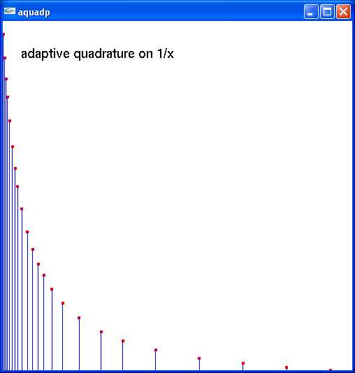
Notice how the method failed with xmin=0.0001, maxed out on storage.
Yes, a better data structure would be a tree or linked list.
It can be made recursive yet that may not be a good idea.
(Programs die from stack overflow!)
On one case the adaptive quadrature used the bins shown in the figure:
Here is a simple implementation of adaptive quadrature, in "C"
/* aquad.c adaptive quadrature numerical integration */
/* for a desired accuracy on irregular functions. */
/* define the function to be integrated as: */
/* double f(double x) */
/* { */
/* // compute value */
/* return value; */
/* } */
/* */
/* integrate from xmin to xmax */
/* approximate desired absolute error in all intervals, eps */
/* accuracy absolutely not guaranteed */
#undef abs
#define abs(x) ((x)<0.0?(-(x)):(x))
double aquad(double f(double x), double xmin, double xmax, double eps)
{
double area, temp, part, h;
double err;
int nmax = 2000;
double sbin[2000]; /* start of bin */
double ebin[2000]; /* end of bin */
double abin[2000]; /* area of bin , sum of these is area */
int fbin[2000]; /* flag, 1 for this bin finished */
int i, j, k, n, nn, done;
int kmax = 20; /* maximum number of times to divide a bin */
n=32; /* initial number of bins */
h = (xmax-xmin)/(double)n;
for(i=0; i<n; i++)
{
sbin[i] = xmin+i*h;
ebin[i] = xmin+(i+1)*h;
fbin[i] = 0;
}
k = 0;
done = 0;
nn = n; /* next available bin */
while(!done)
{
done = 1;
k++;
if(k>=kmax) break; /* quit if more than kmax subdivisions */
area = 0.0;
for(i=0; i<n; i++)
{
if(fbin[i]==1) /* this interval finished */
{
area = area + abin[i]; /* accumulate total area each pass */
continue;
}
temp = f((sbin[i]+ebin[i])/2.0); /* two integration methods */
part = f((3.0*sbin[i]+ebin[i])/4.0);
part = part + f((sbin[i]+3.0*ebin[i])/4.0);
abin[i] = (part+2.0*temp)*(ebin[i]-sbin[i])/4.0;
area = area + abin[i];
err = abs(temp-part/2.0);
if(err*1.414 < eps) /* heuristic */
{
fbin[i] = 1; /* this interval finished */
}
else
{
done = 0; /* must keep dividing */
if(nn>=nmax) /* out of space, quit */
{
done = 1;
for(j=i+1; j<n; j++) area = area + abin[j];
break; /* result not correct */
}
else /* divide interval into two halves */
{
sbin[nn] = (sbin[i]+ebin[i])/2.0;
ebin[nn] = ebin[i];
fbin[nn] = 0;
ebin[i] = sbin[nn];
nn++;
}
}
} /* end for i */
n = nn;
} /* end while */
return area;
} /* end aquad.c */
The results of integrating 1/x for various xmin to xmax are:
(This output linked with aquadt.c that has extra printout.)
test_aquad.c testing aquad.c 1/x eps=0.001
75 intervals, 354 funeval, 6 divides, small=0.101855, maxerr=0.000209298
xmin=0.1, xmax=2, area=2.99538, exact=2.99573, err=-0.000347413
261 intervals, 1470 funeval, 11 divides, small=0.0100607, maxerr=0.000228422
xmin=0.01, xmax=2, area=5.29793, exact=5.29832, err=-0.000390239
847 intervals, 4986 funeval, 16 divides, small=0.00100191, maxerr=0.000226498
xmin=0.001, xmax=2, area=7.6005, exact=7.6009, err=-0.000399734
2000 intervals, 9810 funeval, 18 divides, small=0.000100238, maxerr=0.0141083
xmin=0.0001, xmax=2, area=9.78679, exact=9.90349, err=-0.116702
2000 intervals, 9444 funeval, 17 divides, small=1.04768e-05, maxerr=49.455
xmin=1e-05, xmax=2, area=11.2703, exact=12.2061, err=-0.935768
1.0/((x-0.3)*(x-0.3)+0.01) + 1.0/((x-0.9)*(x-0.9)+0.04) -6
387 intervals, 2226 funeval, 6 divides, small=0.00390625, maxerr=0.000595042
xmin=0, xmax=1, area=29.8582, exact=29.8583, err=-0.000113173
test_aquad.c finished
Notice how the method failed with xmin=0.0001, maxed out on storage.
Yes, a better data structure would be a tree or linked list.
It can be made recursive yet that may not be a good idea.
(Programs die from stack overflow!)
On one case the adaptive quadrature used the bins shown in the figure:
 On some bigger problems, I had run starting with n = 8;
This missed the area where the slope was large.
Just like using the steepest descent method for finding roots,
you may hit a local flat area and miss the part that should
be adaptive.
The above was to demonstrate the "bins" and used way too much
memory. The textbook has pseudo code on Page 301 that uses
much less storage. A modified version of that code is:
/* aquad3.c from book page 301, with modifications */
#undef abs
#define abs(a) ((a)<0.0?(-(a)):(a))
static double stack[100][7]; /* a place to store/retrieve */
static int top, maxtop; /* top points to where stored */
void store(double s0, double s1, double s2, double s3, double s4,
double s5, double s6)
{
stack[top][0] = s0;
stack[top][1] = s1;
stack[top][2] = s2;
stack[top][3] = s3;
stack[top][4] = s4;
stack[top][5] = s5;
stack[top][6] = s6;
}
void retrieve(double* s0, double* s1, double* s2, double* s3, double* s4,
double* s5, double* s6)
{
*s0 = stack[top][0];
*s1 = stack[top][1];
*s2 = stack[top][2];
*s3 = stack[top][3];
*s4 = stack[top][4];
*s5 = stack[top][5];
*s6 = stack[top][6];
} /* end retrieve */
double Sn(double F0, double F1, double F2, double h)
{
return h*(F0 + 4.0*F1 + F2)/3.0; /* error term 2/90 h^3 f^(3)(c) */
} /* end Sn */
double RS(double F0, double F1, double F2, double F3,
double F4, double h)
{
return h*(14.0*F0 +64.0*F1 + 24.0*F2 + 64.0*F3 + 14.0*F4)/45.0;
/* error term 8/945 h^7 f^(8)(c) */
} /* end RS */
double aquad3(double f(double x), double xmin, double xmax, double eps)
{
double a, b, c, d, e;
double Fa, Fb, Fc, Fd, Fe;
double h1, h2, hmin;
double Sab, Sac, Scb, S2ab;
double tol; /* eps */
double val, value;
maxtop = 99;
top = 0;
value = 0.0;
tol = eps;
a = xmin;
b = xmax;
h1 = (b-a)/2.0;
c = a + h1;
Fa = f(a);
Fc = f(c);
Fb = f(b);
Sab = Sn(Fa, Fc, Fb, h1);
store(a, Fa, Fc, Fb, h1, tol, Sab);
top = 1;
while(top > 0)
{
top--;
retrieve(&a, &Fa, &Fc, &Fb, &h1, &tol, &Sab);
c = a + h1;
b = a + 2.0*h1;
h2 = h1/2;
d = a + h2;
e = a + 3.0*h2;
Fd = f(d);
Fe = f(e);
Sac = Sn(Fa, Fd, Fc, h2);
Scb = Sn(Fc, Fe, Fb, h2);
S2ab = Sac + Scb;
if(abs(S2ab-Sab) < tol)
{
val = RS(Fa, Fd, Fc, Fe, Fb, h2);
value = value + val;
}
else
{
h1 = h2;
tol = tol/2.0;
store(a, Fa, Fd, Fc, h1, tol, Sac);
top++;
store(c, Fc, Fe, Fb, h1, tol, Scb);
top++;
}
if(top>=maxtop) break;
} /* end while */
return value;
} /* end main of aquad3.c */
The same test cases, using aquad3t.c, gave the following result:
test_aquad3.c testing aquad3.c 1/x eps=0.001
aquad3 hitop=3, funeval=45, hmin=0.0148437
xmin=0.1, xmax=2, area=2.99573, exact=2.99573, err=9.25606e-07
aquad3 hitop=3, funeval=109, hmin=0.00048584
xmin=0.01, xmax=2, area=5.29832, exact=5.29832, err=1.50725e-06
aquad3 hitop=4, funeval=221, hmin=3.05023e-05
xmin=0.001, xmax=2, area=7.6009, exact=7.6009, err=1.65548e-06
aquad3 hitop=5, funeval=425, hmin=1.90725e-06
xmin=0.0001, xmax=2, area=9.90349, exact=9.90349, err=1.66753e-06
aquad3 hitop=6, funeval=777, hmin=1.19209e-07
xmin=1e-05, xmax=2, area=12.2061, exact=12.2061, err=1.66972e-06
1.0/((x-0.3)*(x-0.3)+0.01) + 1.0/((x-0.9)*(x-0.9)+0.04) -6
aquad3 hitop=5, funeval=121, hmin=0.0078125
xmin=0, xmax=1, area=29.8583, exact=29.8583, err=-1.6204e-06
test_aquad3.c finished
More accurate integration by yet another method:
This uses equally spaced points and gets more accuracy
by using more values of the function being integrated,
F0, F1, F2, ... (the first aquad above used h and 2h,
the aquad3 used 2h and 4h)
On some bigger problems, I had run starting with n = 8;
This missed the area where the slope was large.
Just like using the steepest descent method for finding roots,
you may hit a local flat area and miss the part that should
be adaptive.
The above was to demonstrate the "bins" and used way too much
memory. The textbook has pseudo code on Page 301 that uses
much less storage. A modified version of that code is:
/* aquad3.c from book page 301, with modifications */
#undef abs
#define abs(a) ((a)<0.0?(-(a)):(a))
static double stack[100][7]; /* a place to store/retrieve */
static int top, maxtop; /* top points to where stored */
void store(double s0, double s1, double s2, double s3, double s4,
double s5, double s6)
{
stack[top][0] = s0;
stack[top][1] = s1;
stack[top][2] = s2;
stack[top][3] = s3;
stack[top][4] = s4;
stack[top][5] = s5;
stack[top][6] = s6;
}
void retrieve(double* s0, double* s1, double* s2, double* s3, double* s4,
double* s5, double* s6)
{
*s0 = stack[top][0];
*s1 = stack[top][1];
*s2 = stack[top][2];
*s3 = stack[top][3];
*s4 = stack[top][4];
*s5 = stack[top][5];
*s6 = stack[top][6];
} /* end retrieve */
double Sn(double F0, double F1, double F2, double h)
{
return h*(F0 + 4.0*F1 + F2)/3.0; /* error term 2/90 h^3 f^(3)(c) */
} /* end Sn */
double RS(double F0, double F1, double F2, double F3,
double F4, double h)
{
return h*(14.0*F0 +64.0*F1 + 24.0*F2 + 64.0*F3 + 14.0*F4)/45.0;
/* error term 8/945 h^7 f^(8)(c) */
} /* end RS */
double aquad3(double f(double x), double xmin, double xmax, double eps)
{
double a, b, c, d, e;
double Fa, Fb, Fc, Fd, Fe;
double h1, h2, hmin;
double Sab, Sac, Scb, S2ab;
double tol; /* eps */
double val, value;
maxtop = 99;
top = 0;
value = 0.0;
tol = eps;
a = xmin;
b = xmax;
h1 = (b-a)/2.0;
c = a + h1;
Fa = f(a);
Fc = f(c);
Fb = f(b);
Sab = Sn(Fa, Fc, Fb, h1);
store(a, Fa, Fc, Fb, h1, tol, Sab);
top = 1;
while(top > 0)
{
top--;
retrieve(&a, &Fa, &Fc, &Fb, &h1, &tol, &Sab);
c = a + h1;
b = a + 2.0*h1;
h2 = h1/2;
d = a + h2;
e = a + 3.0*h2;
Fd = f(d);
Fe = f(e);
Sac = Sn(Fa, Fd, Fc, h2);
Scb = Sn(Fc, Fe, Fb, h2);
S2ab = Sac + Scb;
if(abs(S2ab-Sab) < tol)
{
val = RS(Fa, Fd, Fc, Fe, Fb, h2);
value = value + val;
}
else
{
h1 = h2;
tol = tol/2.0;
store(a, Fa, Fd, Fc, h1, tol, Sac);
top++;
store(c, Fc, Fe, Fb, h1, tol, Scb);
top++;
}
if(top>=maxtop) break;
} /* end while */
return value;
} /* end main of aquad3.c */
The same test cases, using aquad3t.c, gave the following result:
test_aquad3.c testing aquad3.c 1/x eps=0.001
aquad3 hitop=3, funeval=45, hmin=0.0148437
xmin=0.1, xmax=2, area=2.99573, exact=2.99573, err=9.25606e-07
aquad3 hitop=3, funeval=109, hmin=0.00048584
xmin=0.01, xmax=2, area=5.29832, exact=5.29832, err=1.50725e-06
aquad3 hitop=4, funeval=221, hmin=3.05023e-05
xmin=0.001, xmax=2, area=7.6009, exact=7.6009, err=1.65548e-06
aquad3 hitop=5, funeval=425, hmin=1.90725e-06
xmin=0.0001, xmax=2, area=9.90349, exact=9.90349, err=1.66753e-06
aquad3 hitop=6, funeval=777, hmin=1.19209e-07
xmin=1e-05, xmax=2, area=12.2061, exact=12.2061, err=1.66972e-06
1.0/((x-0.3)*(x-0.3)+0.01) + 1.0/((x-0.9)*(x-0.9)+0.04) -6
aquad3 hitop=5, funeval=121, hmin=0.0078125
xmin=0, xmax=1, area=29.8583, exact=29.8583, err=-1.6204e-06
test_aquad3.c finished
More accurate integration by yet another method:
This uses equally spaced points and gets more accuracy
by using more values of the function being integrated,
F0, F1, F2, ... (the first aquad above used h and 2h,
the aquad3 used 2h and 4h)
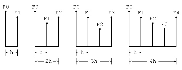 For case h, area = h(F0 + F1)/2
error = 1/12 h f''(c)
For case 2h, area = 2h(F0 + 4F1 + F2)/6
error = 2/90 h^3 f''''(c)
For case 3h, area = 3h(F0 + 3F1 + 3F2 + F3)/8
error = ? h^5 f'^(6)(c)
For case 4h, area = 4h(14F0 + 64F1 + 24F2 + 64F3 + 14F4)/180
error = 8/945 h^7 f'^(8)(c) eighth derivative, c is largest value
Then, the MatLab version:
% test_aquad.m 1/x eps = 0.001
function test_aquad
fid = fopen('test_aquad_m.out', 'w');
eps=0.001;
fprintf(fid, 'test_aquad.m running eps=%g\n', eps);
sprintf('generating test_aquad_m.out \n')
xmin = 0.1;
xmax = 2.0;
q = quad(@f,xmin,xmax,eps);
e = log(xmax)-log(xmin);
fprintf(fid,'xmin=%g, mmax=%g, area=%g, exact=%g, err=%g \n', xmin, xmax, e, q, e-q);
xmin = 0.01;
xmax = 2.0;
q = quad(@f,xmin,xmax,eps);
e = log(xmax)-log(xmin);
fprintf(fid,'xmin=%g, mmax=%g, area=%g, exact=%g, err=%g \n', xmin, xmax, e, q, e-q);
xmin = 0.001;
xmax = 2.0;
q = quad(@f,xmin,xmax,eps);
e = log(xmax)-log(xmin);
fprintf(fid,'xmin=%g, mmax=%g, area=%g, exact=%g, err=%g \n', xmin, xmax, e, q, e-q);
xmin = 0.0001;
xmax = 2.0;
q = quad(@f,xmin,xmax,eps);
e = log(xmax)-log(xmin);
fprintf(fid,'xmin=%g, mmax=%g, area=%g, exact=%g, err=%g \n', xmin, xmax, e, q, e-q);
xmin = 0.000001;
xmax = 2.0;
q = quad(@f,xmin,xmax,eps);
e = log(xmax)-log(xmin);
fprintf(fid,'xmin=%g, mmax=%g, area=%g, exact=%g, err=%g \n', xmin, xmax, e, q, e-q);
fprintf(fid,'1.0/((x-0.3)*(x-0.3)+0.01) + 1.0/((x-0.9).*(x-0.9)+0.04) -6\n');
xmin = 0.0;
xmax = 1.0;
q = quad(@f1,xmin,xmax,eps);
e = 29.8583;
fprintf(fid,'xmin=%g, mmax=%g, area=%g, exact=%g, err=%g \n', xmin, xmax, e, q, e-q);
fprintf(fid,'test_aquad.m finished\n');
return;
function y=f1(x)
y=1.0 ./ ((x-0.3) .*(x-0.3)+0.01) + 1.0 ./ ((x-0.9).*(x-0.9)+0.04) -6.0;
return
end
function y=f(x)
y = 1.0 ./ x;
return
end
end
with results:
test_aquad.m running eps=0.001
xmin=0.1, mmax=2, area=2.99573, exact=2.99597, err=-0.000241595
xmin=0.01, mmax=2, area=5.29832, exact=5.29899, err=-0.000668946
xmin=0.001, mmax=2, area=7.6009, exact=7.60218, err=-0.0012822
xmin=0.0001, mmax=2, area=9.90349, exact=9.90415, err=-0.000660689
xmin=1e-06, mmax=2, area=14.5087, exact=14.5101, err=-0.00148357
1.0/((x-0.3)*(x-0.3)+0.01) + 1.0/((x-0.9).*(x-0.9)+0.04) -6
xmin=0, mmax=1, area=29.8583, exact=29.8583, err=-8.17859e-06
test_aquad.m finished
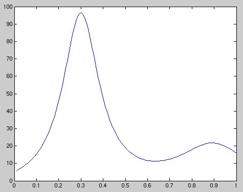
The last case used the curve
y = 1.0/((x-0.3)*(x-0.3)+0.01) + 1.0/((x-0.9)*(x-0.9)+0.04) -6
that looks like:
For case h, area = h(F0 + F1)/2
error = 1/12 h f''(c)
For case 2h, area = 2h(F0 + 4F1 + F2)/6
error = 2/90 h^3 f''''(c)
For case 3h, area = 3h(F0 + 3F1 + 3F2 + F3)/8
error = ? h^5 f'^(6)(c)
For case 4h, area = 4h(14F0 + 64F1 + 24F2 + 64F3 + 14F4)/180
error = 8/945 h^7 f'^(8)(c) eighth derivative, c is largest value
Then, the MatLab version:
% test_aquad.m 1/x eps = 0.001
function test_aquad
fid = fopen('test_aquad_m.out', 'w');
eps=0.001;
fprintf(fid, 'test_aquad.m running eps=%g\n', eps);
sprintf('generating test_aquad_m.out \n')
xmin = 0.1;
xmax = 2.0;
q = quad(@f,xmin,xmax,eps);
e = log(xmax)-log(xmin);
fprintf(fid,'xmin=%g, mmax=%g, area=%g, exact=%g, err=%g \n', xmin, xmax, e, q, e-q);
xmin = 0.01;
xmax = 2.0;
q = quad(@f,xmin,xmax,eps);
e = log(xmax)-log(xmin);
fprintf(fid,'xmin=%g, mmax=%g, area=%g, exact=%g, err=%g \n', xmin, xmax, e, q, e-q);
xmin = 0.001;
xmax = 2.0;
q = quad(@f,xmin,xmax,eps);
e = log(xmax)-log(xmin);
fprintf(fid,'xmin=%g, mmax=%g, area=%g, exact=%g, err=%g \n', xmin, xmax, e, q, e-q);
xmin = 0.0001;
xmax = 2.0;
q = quad(@f,xmin,xmax,eps);
e = log(xmax)-log(xmin);
fprintf(fid,'xmin=%g, mmax=%g, area=%g, exact=%g, err=%g \n', xmin, xmax, e, q, e-q);
xmin = 0.000001;
xmax = 2.0;
q = quad(@f,xmin,xmax,eps);
e = log(xmax)-log(xmin);
fprintf(fid,'xmin=%g, mmax=%g, area=%g, exact=%g, err=%g \n', xmin, xmax, e, q, e-q);
fprintf(fid,'1.0/((x-0.3)*(x-0.3)+0.01) + 1.0/((x-0.9).*(x-0.9)+0.04) -6\n');
xmin = 0.0;
xmax = 1.0;
q = quad(@f1,xmin,xmax,eps);
e = 29.8583;
fprintf(fid,'xmin=%g, mmax=%g, area=%g, exact=%g, err=%g \n', xmin, xmax, e, q, e-q);
fprintf(fid,'test_aquad.m finished\n');
return;
function y=f1(x)
y=1.0 ./ ((x-0.3) .*(x-0.3)+0.01) + 1.0 ./ ((x-0.9).*(x-0.9)+0.04) -6.0;
return
end
function y=f(x)
y = 1.0 ./ x;
return
end
end
with results:
test_aquad.m running eps=0.001
xmin=0.1, mmax=2, area=2.99573, exact=2.99597, err=-0.000241595
xmin=0.01, mmax=2, area=5.29832, exact=5.29899, err=-0.000668946
xmin=0.001, mmax=2, area=7.6009, exact=7.60218, err=-0.0012822
xmin=0.0001, mmax=2, area=9.90349, exact=9.90415, err=-0.000660689
xmin=1e-06, mmax=2, area=14.5087, exact=14.5101, err=-0.00148357
1.0/((x-0.3)*(x-0.3)+0.01) + 1.0/((x-0.9).*(x-0.9)+0.04) -6
xmin=0, mmax=1, area=29.8583, exact=29.8583, err=-8.17859e-06
test_aquad.m finished
The last case used the curve
y = 1.0/((x-0.3)*(x-0.3)+0.01) + 1.0/((x-0.9)*(x-0.9)+0.04) -6
that looks like:
 Passing a function as an argument in Python is easy:
# test_aquad3.py
from aquad3 import aquad3
xmin = 1.0
xmax = 2.0
eps = 0.001
def f(x):
return x*x
print "test_aquad3.py running"
area=aquad3(f, xmin, xmax, eps) # aquad3 compiled alone
print "aquad3(f, xmin, xmax, eps) =", area
With Java, some extra is needed to pass a user function to
a pre written integration class.
You need an interface to the function:
lib_funct.java
The user then provides an implementation to the function
to pass to the integration method and may provide values:
pass_funct.java
The pre written integration, trapezoidal method example,
has the numeric code, yet does not know the function (yet):
main_funct.java
main_funct.out
Then, a hack of test_aquad.c to test_aquad.java using just x^2
test_aquad.java
test_aquad_java.out
Another example with a two parameter function is:
(The Runga-Kutta method of integration is covered in Lecture 26.
This just shown the interface can be more general.)
You need an interface to the function:
RKlib.java
The user then provides an implementation to the function
to pass to the integration method and may provide values:
RKuser.java
The pre written integration method example,
has the numeric code, yet does not know the function (yet):
RKmain.java
RKmain.out
Passing a function as an argument in Python is easy:
# test_aquad3.py
from aquad3 import aquad3
xmin = 1.0
xmax = 2.0
eps = 0.001
def f(x):
return x*x
print "test_aquad3.py running"
area=aquad3(f, xmin, xmax, eps) # aquad3 compiled alone
print "aquad3(f, xmin, xmax, eps) =", area
With Java, some extra is needed to pass a user function to
a pre written integration class.
You need an interface to the function:
lib_funct.java
The user then provides an implementation to the function
to pass to the integration method and may provide values:
pass_funct.java
The pre written integration, trapezoidal method example,
has the numeric code, yet does not know the function (yet):
main_funct.java
main_funct.out
Then, a hack of test_aquad.c to test_aquad.java using just x^2
test_aquad.java
test_aquad_java.out
Another example with a two parameter function is:
(The Runga-Kutta method of integration is covered in Lecture 26.
This just shown the interface can be more general.)
You need an interface to the function:
RKlib.java
The user then provides an implementation to the function
to pass to the integration method and may provide values:
RKuser.java
The pre written integration method example,
has the numeric code, yet does not know the function (yet):
RKmain.java
RKmain.out
Now 3D integration
Matlab
integrate_volume.m source code
integrate_volume_m.out output
using different function definition format:
integrate_volume2.m source code
integrate_volume2_m.out output
Java very accurate using gaulegf
test_gaulegf3D.java source code
test_gaulegf3D_java.out output
Less accurate using trap and other methods
integrate_volume.java source code
integrate_volume_java.out output
integrate_volume.txt calculus
The files are:
test_aquad.c
aquad.h
aquad.c teaching version, do not use
aquadt.c
test_aquad_c.out
test_aquad3.c
aquad3.h
aquad3.c C implementation
test_aquad3_c.out
aquad3t.c
test_aquad3t_c.out
test_aquad.m MatLab builtin
test_aquad_m.out
test_aquad3.f90
aquad3.f90 Fortran 95 implementation
test_aquad3_f90.out
test_aquad3.adb
aquad.ads
aquad.adb Ada 95 implementation
f.adb
f1.adb
test_aquad3_ada.out
lib_funct.java
pass_funct.java
main_funct.java
test_aquad.java
test_aquad_java.out
test_passing_function.py
test_passing_function_py.out
test_aquad3.py
aquad3.py
test_aquad3_py.out
<- previous index next ->
-
CMSC 455 home page
-
Syllabus - class dates and subjects, homework dates, reading assignments
-
Homework assignments - the details
-
Projects -
-
Partial Lecture Notes, one per WEB page
-
Partial Lecture Notes, one big page for printing
-
Downloadable samples, source and executables
-
Some brief notes on Matlab
-
Some brief notes on Python
-
Some brief notes on Fortran 95
-
Some brief notes on Ada 95
-
An Ada math library (gnatmath95)
-
Finite difference approximations for derivatives
-
MATLAB examples, some ODE, some PDE
-
parallel threads examples
-
Reference pages on Taylor series, identities,
coordinate systems, differential operators
-
selected news related to numerical computation