<- previous index next ->
Extending PDE's in polar, cylindrical, spherical
solve PDE in polar coordinates
∇2U(r,Θ) + U(r,Θ) = f(r,Θ)
given Dirichlet boundary values and f
Development version with much checking:
pde_polar_eq.adb
pde_polar_eq_ada.out
solve PDE in cylindrical coordinates
∇2U(r,Θ,z) + U(r,Θ,z) = f(r,Θ,z)
given Dirichlet boundary values and f
reference equations, cylindrical, spherical
Theta and Phi reversed from my programs.
Del_in_cylindrical_and_spherical_coordinates
Development version with much checking:
check_cylinder_deriv.c
check_cylinder_deriv_c.out
pde_cylinderical_eq.c
pde_cylinderical_eq_c.out
check_cylinder_deriv.java
check_cylinder_deriv_java.out
pde_cylinderical_eq.java
pde_cylinderical_eq_java.out
check_cylinder_deriv.adb
check_cylinder_deriv_ada.out
pde_cylinderical_eq.adb
pde_cylinderical_eq_ada.out
solve PDE in spherical coordinates
∇2U(r,Θ,Φ) + U(r,Θ,Φ) = f(r,Θ,Φ)
given Dirichlet boundary values and f
Development versions with much checking:
check_sphere_deriv.c
check_sphere_deriv_c.out
pde_spherical_eq.c
pde_spherical_eq_c.out
check_sphere_deriv.java
check_sphere_deriv_java.out
check_sphere_deriv.adb
check_sphere_deriv_ada.out
check_sphere_deriv.adb
check_sphere_deriv_ada.out
pde_spherical_eq.adb
pde_spherical_eq_ada.out
pde_spherical_eq.f90
pde_spherical_eq_f90.out
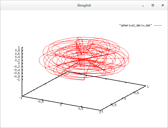
Another set using spherical laplacian
spherical_deriv.java
spherical_deriv_java.out
spherical_pde.mws Maple input
spherical_pde_mws.out Maple output
spherical_deriv.sh gnuplot
spherical_deriv.plot gnuplot
spherical_deriv.dat gnuplot data
 Other utility files needed by sample code above:
simeq.h
simeq.c
nuderiv.h
nuderiv.c
simeq.java
nuderiv.java
simeqb.adb
nuderiv.adb
nuderiv.f90
inverse.f90
May be converted to other languages.
Also possible, other toroidal coordinates.
Other utility files needed by sample code above:
simeq.h
simeq.c
nuderiv.h
nuderiv.c
simeq.java
nuderiv.java
simeqb.adb
nuderiv.adb
nuderiv.f90
inverse.f90
May be converted to other languages.
Also possible, other toroidal coordinates.
Spherical Laplacian in higher dimensions, 4 and 8 tested
// nabla.c del^2 = nabla = Laplacian n dimensional space of function U(r,a)
// n-dimensional sphere, radius r
// a[0],...,a[n-2] are angles in radians (User can rename in their code)
// compute Laplacian of U(r,a) at given angles
// double nabla(int n, double r, double a[], double (*U()));
//
// alternate call if partial derivative values of U are known
// da[0],...,da[n-2] are first partial derivatives of users U(r,a)
// dda[0],...,dda[n-2] are second partial derivatives of users U(r,a)
// with respect to a[0],...,a[n-2] evaluated
// at a[0],...,a[n-1]
// double nablapd(int n, double r, double a[],
// double dr, double ddr, double da[], double dda[]);
//
// utility function for n-dimensional cartesian to spherical coordinates
// n>3 x[0..n-1] r, a[0..n-2]
// void toSpherical(int n, double x[], double *r, double a[]);
//
// utility function for n-dimensional spherical to cartesian coordinates
// n>3 r, a[0..n-2] x[0..n-1]
// void toCartesian(int n, double r, double a[], double x[]);
//
// utility function for n-dimensional U(r, a) at r, a[]
// to derivatives da[] and dda[]
// void sphereDeriv(int n, double (*U)(), double r, double a[],
// double *dr, double *drr, double da[], double dda[]);
//
// method for basic nabla_n:
// use iterative function, n>3, for computing nabla_n of U(r,a[])
// using d for partial derivative symbol and U for U(r,a[]) and
// adjusting subscripts for a[0],...,a[n-2]
//
// before reduction for numerical computation:
// nabla_n = 1/r^n-1 d(r^n-1 dU/dr)/dr + 1/r^2 L2(n)
//
// after reduction:
// nabla_n = (n-1)/r dU/dr + d^2U/dr^2 + 1/r^2 L2(n, r, a)
//
// in code:
// nabla_n = ((n-1)/r)*dr + ddr + (1.0/(r*r))*L2(n,r,a);
//
// before reduction and adjusting subscripts of a_i code a[]:
// L2(n,r,a) = sum(i=2,n){prod(j=i+1,n){1/sin^2(a_j)} *
// 1/sin(a_i)^(i-2)*d(sin(a_i)^(i-2)*dU/da_i)/da_i}
//
// after reduction:
// L2(n,r,a) = sum(i=2,n){{prod(j=i+1,n){1/sin^2(a_j)} *
// (i-2)*cos(a_i)/sin(a_i) *dU/da_i + d^2U/da_i^2}
//
// after adjusting subscripts:
// L2(n,r,a) = sum(i=2,n){{prod(j=i+1,n){1/sin^2(a_j-2)} *
// ((i-2)*cos(a_i-2)/sin(a_i-2)) * dU/da_i-2 + d^2U/(da_i-2)^2}
//
// in code (n>3):
// tmp = 0.0;
// for(i=2; i<=n; i++)
// {
// ptmp = 1.0;
// for(j=i+1; j<=n; j++)
// {
// ptmp = ptmp * (1.0/sin(a[j-2])*sin(a[j-2]));
// }
// ptmp = ptmp * ((i-2.0)*cos(s[i-2])/sin(a[i-2])) * da[i-2] * dda[i-2];
// tmp = tmp + ptmp;
// }
// L2(n,r,a) = tmp;
//
// example 8 Dimensional sphere, n=8 symmetry with zero based indexing
// x0 = r cos(a0)
// x1 = r sin(a0) cos(a1)
// x2 = r sin(a0) sin(a1) cos(a2)
// x3 = r sin(a0) sin(a1) sin(a2) cos(a3)
// x4 = r sin(a0) sin(a1) sin(a2) sin(a3) cos(a4)
// x5 = r sin(a0) sin(a1) sin(a2) sin(a3) sin(a4) cos(a5)
// x6 = r sin(a0) sin(a1) sin(a2) sin(a3) sin(a4) sin(a5) cos(a6)
// x7 = r sin(a0) sin(a1) sin(a2) sin(a3) sin(a4) sin(a5) sin(a6)
//
// r = sqrt(x0^2 + x1^2 + x2^2 + x3^2 + x4^2 + x5^2 + x6^2 + x7^2)
// a0 = acos(x0/r)
// a1 = acos(x1/sqrt(x1^2 + x2^2 + x3^2 + x4^2 + x5^2 + x6^2 + x7^2))
// a2 = acos(x2/sqrt(x2^2 + x3^2 + x4^2 + x5^2 + x6^2 + x7^2))
// a3 = acos(x3/sqrt(x3^2 + x4^2 + x5^2 + x6^2 + x7^2))
// a4 = acos(x4/sqrt(x4^2 + x5^2 + x6^2 + x7^2))
// a5 = acos(x5/sqrt(x5^2 + x6^2 + x7^2))
// a6 = acos(x6/sqrt(x6^2 + x7^2)) if x7>=0
// a6 = 2Pi-acos(x6/sqrt(x6^2 + x6^2)) if x7<0
nabla.h source code
nabla.c source code
test_nabla.c test source code
test_nabla_c.out test results
test_nabla8.c test source code
test_nabla8_c.out test results
<- previous index next ->
-
CMSC 455 home page
-
Syllabus - class dates and subjects, homework dates, reading assignments
-
Homework assignments - the details
-
Projects -
-
Partial Lecture Notes, one per WEB page
-
Partial Lecture Notes, one big page for printing
-
Downloadable samples, source and executables
-
Some brief notes on Matlab
-
Some brief notes on Python
-
Some brief notes on Fortran 95
-
Some brief notes on Ada 95
-
An Ada math library (gnatmath95)
-
Finite difference approximations for derivatives
-
MATLAB examples, some ODE, some PDE
-
parallel threads examples
-
Reference pages on Taylor series, identities,
coordinate systems, differential operators
-
selected news related to numerical computation