<- previous index next ->
A modified version of fem_50, a Matlab program to use
the Finite Element Method, FEM, to solve a specific
partial differential equation is applied to three very
small test cases with full printout to show the details
of one software implementation.
The differential equation is:
d^2 u(x,y) d^2 u(x,y)
- ---------- - ---------- = f(x,y) or -Uxx(x,y) -Uyy(x,y) = F(x,y)
dx^2 dy^2
For testing, the solution is u(x,y)=1 + 2/11 x^2 + 3/11 y^2
and then f(x,y)= - 10/11
The modified fem_50d.m is also shown below
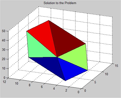
Case 1 used a triangularization with 6 triangles
7 nodes
6 boundary nodes
1 degree of freedom
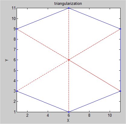 The blue edges and dots are boundary.
The red edges and dots are internal, free.
The one free node is in the center, node number 7.
The full output is A7_fem_50d.out
The solution for the 7 nodes is at the end.
Input files are:
A7_coord.dat
A7_elem3.dat
A7_dirich.dat
The files A7_elem4.dat and A7_neum.dat exists and are empty.
The solution plot is:
The blue edges and dots are boundary.
The red edges and dots are internal, free.
The one free node is in the center, node number 7.
The full output is A7_fem_50d.out
The solution for the 7 nodes is at the end.
Input files are:
A7_coord.dat
A7_elem3.dat
A7_dirich.dat
The files A7_elem4.dat and A7_neum.dat exists and are empty.
The solution plot is:
 Case 2 used a triangularization with 16 triangles
15 nodes
12 boundary nodes
3 degrees of freedom
Case 2 used a triangularization with 16 triangles
15 nodes
12 boundary nodes
3 degrees of freedom
 The blue edges and dots are boundary.
The red edges and dots are internal, free.
The three free nodes are in the center, number 13, 14, 15
The full output is A15_fem_50d.out
The solution for the 15 nodes is at the end.
Input files are:
A15_coord.dat
A15_elem3.dat
A15_dirich.dat
The files A15_elem4.dat and A15_neum.dat exists and are empty.
The solution plot is:
The blue edges and dots are boundary.
The red edges and dots are internal, free.
The three free nodes are in the center, number 13, 14, 15
The full output is A15_fem_50d.out
The solution for the 15 nodes is at the end.
Input files are:
A15_coord.dat
A15_elem3.dat
A15_dirich.dat
The files A15_elem4.dat and A15_neum.dat exists and are empty.
The solution plot is:
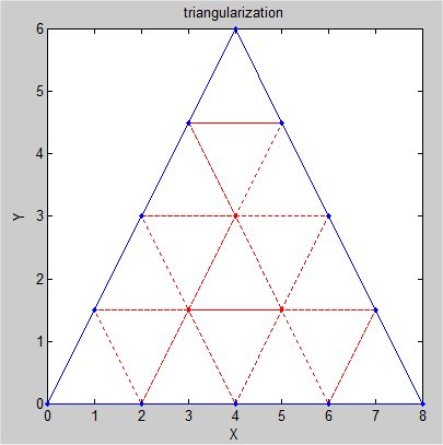
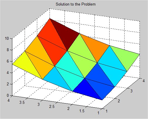
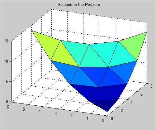 Case 3 used a triangularization with 18 triangles
16 nodes
12 boundary nodes
4 degrees of freedom
Case 3 used a triangularization with 18 triangles
16 nodes
12 boundary nodes
4 degrees of freedom
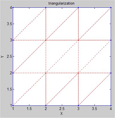 The blue edges and dots are boundary.
The red edges and dots are internal, free.
The four free nodes are in the center, numbered 1, 2, 3, 4
The full output is A16_fem_50d.out
The solution for the 16 nodes is at the end.
Input files are:
A16_coord.dat
A16_elem3.dat
A16_dirich.dat
The files A16_elem4.dat and A16_neum.dat exists and are empty.
The solution plot is:
The blue edges and dots are boundary.
The red edges and dots are internal, free.
The four free nodes are in the center, numbered 1, 2, 3, 4
The full output is A16_fem_50d.out
The solution for the 16 nodes is at the end.
Input files are:
A16_coord.dat
A16_elem3.dat
A16_dirich.dat
The files A16_elem4.dat and A16_neum.dat exists and are empty.
The solution plot is:
 The original fem_50.m all in one file with lots of output added
%% fem_50d applies the finite element method to Laplace's equation.
function fem_50d
% input a prefix, e.g. A7_
% files read A7_coord.dat one x y pair per line, for nodes in order 1, 2, ...
% A7_elem3.dat three node numbers per line, triangles, any order
% function stima3 is applied to these cooddinates
% A7_elem4.dat four node numbers per line, quadralaterals
% function stima4 is applied to these coordinates
% A7_dirich.dat two node numbers per line, dirichlet boundary
% function u_d is applied to these coordinates
% A7_neum.dat two node numbers per line, neumann bounday
% function g is applied to these coordinates
%
% Discussion:
% FEM_50d is a set of MATLAB routines to apply the finite
% element method to solving Laplace's equation in an arbitrary
% region, using about 50 lines of MATLAB code.
%
% FEM_50d is partly a demonstration, to show how little it
% takes to implement the finite element method (at least using
% every possible MATLAB shortcut.) The user supplies datafiles
% that specify the geometry of the region and its arrangement
% into triangular and quadrilateral elements, and the location
% and type of the boundary conditions, which can be any mixture
% of Neumann and dirichlet.
%
% The unknown state variable U(x,y) is assumed to satisfy
% Laplace's equation:
% -Uxx(x,y) - Uyy(x,y) = F(x,y) in Omega
% with dirichlet boundary conditions
% U(x,y) = U_D(x,y) on Gamma_D
% and Neumann boundary conditions on the outward normal derivative:
% Un(x,y) = G(x,y) on Gamma_N
% If Gamma designates the boundary of the region Omega,
% then we presume that
% Gamma = Gamma_D + Gamma_N
% but the user is free to determine which boundary conditions to
% apply. Note, however, that the problem will generally be singular
% unless at least one dirichlet boundary condition is specified.
%
% The code uses piecewise linear basis functions for triangular elements,
% and piecewise isoparametric bilinear basis functions for quadrilateral
% elements.
%
% The user is required to supply a number of data files and MATLAB
% functions that specify the location of nodes, the grouping of nodes
% into elements, the location and value of boundary conditions, and
% the right hand side function in Laplace's equation. Note that the
% fact that the geometry is completely up to the user means that
% just about any two dimensional region can be handled, with arbitrary
% shape, including holes and islands.
%
% Modified:
% 29 March 2004
% 23 February 2008 JSS
% 3 March 2008 JSS
% Reference:
% Jochen Alberty, Carsten Carstensen, Stefan Funken,
% Remarks Around 50 Lines of MATLAB:
% Short Finite Element Implementation,
% Numerical Algorithms,
% Volume 20, pages 117-137, 1999.
%
clear
format compact
prename = input('enter prefix to file names: ', 's')
diary 'fem_50d.out'
disp([prename 'fem_50d.out'])
debug = input('enter debug level:0=none, 1=input and matrices, 2=assembly ')
%
% Read the nodal coordinatesinate data file.
% ordered list of x y pairs, coordinates for nodes
% nodes must be sequentially numbered 1, 2, 3, ...
coordinates = load(strcat(prename,'coord.dat'));
if debug>0
disp([prename 'coord.dat ='])
disp(coordinates)
end % debug
%
% Read the triangular element data file.
% three integer node numbers per line
elements3 = load(strcat(prename,'elem3.dat'));
if debug>0
disp([prename 'elem3.dat ='])
disp(elements3)
end % debug
%
% Read the quadrilateral element data file.
% four integer node numbers per line
elements4 = load(strcat(prename,'elem4.dat'));
if debug>0
disp([prename 'elem4.dat ='])
disp(elements4)
end % debug
%
% Read the dirichlet boundary edge data file.
% two integer node numbers per line, function u_d sets values
% there must be at least one pair
% other boundary edges are set in neumann
dirichlet = load(strcat(prename,'dirich.dat'));
if debug>0
disp([prename 'dirich.dat ='])
disp(dirichlet)
end % debug
%
% Read the Neumann boundary edge data file.
% two integer node numbers per line, function g sets values
neumann = load(strcat(prename,'neum.dat'));
if debug>0
disp([prename 'neum.dat ='])
disp(neumann)
end % debug
A = sparse ( size(coordinates,1), size(coordinates,1) );
b = sparse ( size(coordinates,1), 1 );
%
% Assembly from triangles.
%
for j = 1 : size(elements3,1)
VV = coordinates(elements3(j,:),:);
MM = stima3(coordinates(elements3(j,:),:));
if debug>1
disp(['MM = stima3(VV) at j=' num2str(j) ' nodes(' ...
num2str(elements3(j,1)) ',' num2str(elements3(j,2)) ',' ...
num2str(elements3(j,3)) ')'])
disp('VV=')
disp(VV)
disp('MM=')
disp(MM)
end % debug
A(elements3(j,:),elements3(j,:)) = A(elements3(j,:),elements3(j,:)) + MM;
end
if debug>0
disp('assembly from triangles A=')
disp(A)
end % debug
%
% Assembly from quadralaterals.
%
for j = 1 : size(elements4,1)
VV = coordinates(elements3(j,:),:);
MM = stima4(coordinates(elements4(j,:),:));
if debug>1
disp(['MM = stima3(VV) at j=' num2str(j) ' nodes(' ...
num2str(elements4(j,1)) ',' num2str(elements4(j,2)) ',' ...
num2str(elements4(j,3)) ',' num2str(elements4(j,4)) ')'])
disp('VV=')
disp(VV)
disp('MM=')
disp(MM)
end % debug
A(elements4(j,:),elements4(j,:)) = A(elements4(j,:),elements4(j,:)) + MM;
end
if debug>0
disp('assembly from triangles and rectangles A=')
disp(A)
end % debug
%
% Volume Forces from triangles.
%
for j = 1 : size(elements3,1)
b(elements3(j,:)) = b(elements3(j,:)) ...
+ det( [1,1,1; coordinates(elements3(j,:),:)'] ) * ...
f(sum(coordinates(elements3(j,:),:))/3)/6;
end
if debug>0
disp('forces from triangles b=')
disp(b)
end % debug
%
% Volume Forces from quadralaterals.
%
for j = 1 : size(elements4,1)
b(elements4(j,:)) = b(elements4(j,:)) ...
+ det([1,1,1; coordinates(elements4(j,1:3),:)'] ) * ...
f(sum(coordinates(elements4(j,:),:))/4)/4;
end
if debug>0
disp('forces from triangles and rectangles b=')
disp(b)
end % debug
%
% Neumann conditions.
%
for j = 1 : size(neumann,1)
GG = norm(coordinates(neumann(j,1),:) - coordinates(neumann(j,2),:)) * ...
g(sum(coordinates(neumann(j,:),:))/2)/2;
if debug>2
disp(['Neumann at j=' num2str(j)])
disp(GG)
end % debug
b(neumann(j,:)) = b(neumann(j,:)) + GG
end
if debug>0
disp('using g() add neumann conditions b=')
disp(b)
end % debug
%
% Determine which nodes are associated with dirichlet conditions.
% Assign the corresponding entries of U, and adjust the right hand side.
%
u = sparse ( size(coordinates,1), 1 );
BoundNodes = unique ( dirichlet );
if debug>1
disp('BoundNodes=')
disp(BoundNodes)
end % debug
u(BoundNodes) = u_d ( coordinates(BoundNodes,:) );
if debug>0
disp('using u_d() add dirichlet conditions u=')
disp(u)
end % debug
b = b - A * u;
if debug>0
disp('apply u to b, dirichlet conditions b=')
disp(b)
end % debug
%
% Compute the solution by solving A * u = b
% for the, un bound, remaining unknown values of u.
%
FreeNodes = setdiff ( 1:size(coordinates,1), BoundNodes );
u(FreeNodes) = A(FreeNodes,FreeNodes) \ b(FreeNodes);
if debug>0
disp('solve for A * u = b u=')
disp(u)
end % debug
%
% Graphic representation.
%
show ( elements3, elements4, coordinates, full(u), dirichlet );
%
% check solution
%
for i=1:size(coordinates,1)
disp([num2str(i) ' x= ' num2str(coordinates(i,1)) ' y= ' num2str(coordinates(i,2)) ...
' analytic solution= ' num2str(uana(coordinates(i,1),coordinates(i,2)))])
end
diary off
return % logical end of function fem_50d
%% uana computes boundary values and analytic solution for checking
% Discussion:
% This is generally unknown yet is used here for testing
% Parameters:
% Input, real pair xx,yy are x,y coordinates
% Output, value of solution at x,y
%
function ana = uana(xx, yy)
ana= 1.0+(2.0/11.0)*xx*xx+(3.0/11.0)*yy*yy;
end % uana
%% f evaluates the right hand side of Laplace's equation.
% Discussion:
% This routine must be changed by the user to reflect a particular problem.
% Parameters:
% Input, real U(N,M), contains the M-dimensional coordinates of N points.
% Output, VALUE(N), contains the value of the right hand side of Laplace's
% equation at each of the points.
function valuef = f ( uf )
valuef = ones ( size ( uf, 1 ), 1 );
valuef = valuef.*(-10/11.0);
end % f
%% g evaluates the outward normal values assigned at Neumann boundary conditions.
% Discussion:
% This routine must be changed by the user to reflect a particular problem.
% Parameters:
% Input, real U(N,M), contains the M-dimensional coordinates of N points.
% Output, VALUE(N), contains the value of outward normal at each point
% where a Neumann boundary condition is applied.
function valueg = g ( ug )
valueg = zeros ( size ( ug, 1 ), 1 );
end % g
%% u_d evaluates the dirichlet boundary conditions.
% Discussion:
% The user must supply the appropriate routine for a given problem
% Parameters:
% Input, real U(N,M), contains the M-dimensional coordinates of N points.
% Output, VALUE(N), contains the value of the dirichlet boundary
% condition at each point.
function valued = u_d ( ud )
valued = zeros ( size ( ud, 1 ), 1 );
for kk=1:size(ud,1)
% U(x,y) = 1 + 2/11 x^2 + 3/11 y^2 solution values on boundary
valued(kk)=uana(ud(kk,1),ud(kk,2));
end
end % u_d
%% STIMA3 determines the local stiffness matrix for a triangular element.
% Discussion:
%
% Although this routine is intended for 2D usage, the same formulas
% work for tetrahedral elements in 3D. The spatial dimension intended
% is determined implicitly, from the spatial dimension of the vertices.
% Parameters:
%
% Input, real VERTICES(1:(D+1),1:D), contains the D-dimensional
% coordinates of the vertices.
%
% Output, real M(1:(D+1),1:(D+1)), the local stiffness matrix
% for the element.
function M = stima3 ( vertices )
d = size ( vertices, 2 );
D_eta = [ ones(1,d+1); vertices' ] \ [ zeros(1,d); eye(d) ];
M = det ( [ ones(1,d+1); vertices' ] ) * D_eta * D_eta' / prod ( 1:d );
end % stima3
%% STIMA4 determines the local stiffness matrix for a quadrilateral element.
% Parameters:
% Input, real VERTICES(1:4,1:2), contains the coordinates of the vertices.
% Output, real M(1:4,1:4), the local stiffness matrix for the element.%
function M = stima4 ( vertices )
D_Phi = [ vertices(2,:) - vertices(1,:); vertices(4,:) - vertices(1,:) ]';
B = inv ( D_Phi' * D_Phi );
C1 = [ 2, -2; -2, 2 ] * B(1,1) ...
+ [ 3, 0; 0, -3 ] * B(1,2) ...
+ [ 2, 1; 1, 2 ] * B(2,2);
C2 = [ -1, 1; 1, -1 ] * B(1,1) ...
+ [ -3, 0; 0, 3 ] * B(1,2) ...
+ [ -1, -2; -2, -1 ] * B(2,2);
M = det ( D_Phi ) * [ C1 C2; C2 C1 ] / 6;
end % stima4
%% SHOW displays the solution of the finite element computation.
% Parameters:
% Input, integer elements3(N3,3), the nodes that make up each triangle.
% Input, integer elements4(N4,4), the nodes that make up each quadrilateral.
% Input, real coordinates(N,1:2), the coordinates of each node.
% Input, real U(N), the finite element coefficients which represent the solution.
% There is one coefficient associated with each node.
function show ( elements3, elements4, coordinates, us, dirichlet )
figure(1)
hold off
%
% Display the information associated with triangular elements.
trisurf ( elements3, coordinates(:,1), coordinates(:,2), us' );
%
% Retain the previous image, and overlay the information associated
% with quadrilateral elements.
hold on
trisurf ( elements4, coordinates(:,1), coordinates(:,2), us' );
%
% Define the initial viewing angle.
%
view ( -67.5, 30 );
title ( 'Solution to the Problem' )
hold off
figure(2)
for kk=1:size(elements3,1)
plot([coordinates(elements3(kk,1),1) ...
coordinates(elements3(kk,2),1) ...
coordinates(elements3(kk,3),1) ...
coordinates(elements3(kk,1),1)], ...
[coordinates(elements3(kk,1),2) ...
coordinates(elements3(kk,2),2) ...
coordinates(elements3(kk,3),2) ...
coordinates(elements3(kk,1),2)],':r')
hold on
end
for kk=1:size(dirichlet,1)
plot([coordinates(dirichlet(kk,1),1) ...
coordinates(dirichlet(kk,2),1)], ...
[coordinates(dirichlet(kk,1),2) ...
coordinates(dirichlet(kk,2),2)],'-b')
hold on
end
title('triangularization')
xlabel('X')
ylabel('Y')
axis tight
axis square
grid off
hold on
xb=coordinates(BoundNodes,1);
yb=coordinates(BoundNodes,2);
plot(xb,yb,'.b')
hold on
xb=coordinates(FreeNodes,1);
yb=coordinates(FreeNodes,2);
plot(xb,yb,'.r')
hold off
end % show
end % fem_50d
The original fem_50.m all in one file with lots of output added
%% fem_50d applies the finite element method to Laplace's equation.
function fem_50d
% input a prefix, e.g. A7_
% files read A7_coord.dat one x y pair per line, for nodes in order 1, 2, ...
% A7_elem3.dat three node numbers per line, triangles, any order
% function stima3 is applied to these cooddinates
% A7_elem4.dat four node numbers per line, quadralaterals
% function stima4 is applied to these coordinates
% A7_dirich.dat two node numbers per line, dirichlet boundary
% function u_d is applied to these coordinates
% A7_neum.dat two node numbers per line, neumann bounday
% function g is applied to these coordinates
%
% Discussion:
% FEM_50d is a set of MATLAB routines to apply the finite
% element method to solving Laplace's equation in an arbitrary
% region, using about 50 lines of MATLAB code.
%
% FEM_50d is partly a demonstration, to show how little it
% takes to implement the finite element method (at least using
% every possible MATLAB shortcut.) The user supplies datafiles
% that specify the geometry of the region and its arrangement
% into triangular and quadrilateral elements, and the location
% and type of the boundary conditions, which can be any mixture
% of Neumann and dirichlet.
%
% The unknown state variable U(x,y) is assumed to satisfy
% Laplace's equation:
% -Uxx(x,y) - Uyy(x,y) = F(x,y) in Omega
% with dirichlet boundary conditions
% U(x,y) = U_D(x,y) on Gamma_D
% and Neumann boundary conditions on the outward normal derivative:
% Un(x,y) = G(x,y) on Gamma_N
% If Gamma designates the boundary of the region Omega,
% then we presume that
% Gamma = Gamma_D + Gamma_N
% but the user is free to determine which boundary conditions to
% apply. Note, however, that the problem will generally be singular
% unless at least one dirichlet boundary condition is specified.
%
% The code uses piecewise linear basis functions for triangular elements,
% and piecewise isoparametric bilinear basis functions for quadrilateral
% elements.
%
% The user is required to supply a number of data files and MATLAB
% functions that specify the location of nodes, the grouping of nodes
% into elements, the location and value of boundary conditions, and
% the right hand side function in Laplace's equation. Note that the
% fact that the geometry is completely up to the user means that
% just about any two dimensional region can be handled, with arbitrary
% shape, including holes and islands.
%
% Modified:
% 29 March 2004
% 23 February 2008 JSS
% 3 March 2008 JSS
% Reference:
% Jochen Alberty, Carsten Carstensen, Stefan Funken,
% Remarks Around 50 Lines of MATLAB:
% Short Finite Element Implementation,
% Numerical Algorithms,
% Volume 20, pages 117-137, 1999.
%
clear
format compact
prename = input('enter prefix to file names: ', 's')
diary 'fem_50d.out'
disp([prename 'fem_50d.out'])
debug = input('enter debug level:0=none, 1=input and matrices, 2=assembly ')
%
% Read the nodal coordinatesinate data file.
% ordered list of x y pairs, coordinates for nodes
% nodes must be sequentially numbered 1, 2, 3, ...
coordinates = load(strcat(prename,'coord.dat'));
if debug>0
disp([prename 'coord.dat ='])
disp(coordinates)
end % debug
%
% Read the triangular element data file.
% three integer node numbers per line
elements3 = load(strcat(prename,'elem3.dat'));
if debug>0
disp([prename 'elem3.dat ='])
disp(elements3)
end % debug
%
% Read the quadrilateral element data file.
% four integer node numbers per line
elements4 = load(strcat(prename,'elem4.dat'));
if debug>0
disp([prename 'elem4.dat ='])
disp(elements4)
end % debug
%
% Read the dirichlet boundary edge data file.
% two integer node numbers per line, function u_d sets values
% there must be at least one pair
% other boundary edges are set in neumann
dirichlet = load(strcat(prename,'dirich.dat'));
if debug>0
disp([prename 'dirich.dat ='])
disp(dirichlet)
end % debug
%
% Read the Neumann boundary edge data file.
% two integer node numbers per line, function g sets values
neumann = load(strcat(prename,'neum.dat'));
if debug>0
disp([prename 'neum.dat ='])
disp(neumann)
end % debug
A = sparse ( size(coordinates,1), size(coordinates,1) );
b = sparse ( size(coordinates,1), 1 );
%
% Assembly from triangles.
%
for j = 1 : size(elements3,1)
VV = coordinates(elements3(j,:),:);
MM = stima3(coordinates(elements3(j,:),:));
if debug>1
disp(['MM = stima3(VV) at j=' num2str(j) ' nodes(' ...
num2str(elements3(j,1)) ',' num2str(elements3(j,2)) ',' ...
num2str(elements3(j,3)) ')'])
disp('VV=')
disp(VV)
disp('MM=')
disp(MM)
end % debug
A(elements3(j,:),elements3(j,:)) = A(elements3(j,:),elements3(j,:)) + MM;
end
if debug>0
disp('assembly from triangles A=')
disp(A)
end % debug
%
% Assembly from quadralaterals.
%
for j = 1 : size(elements4,1)
VV = coordinates(elements3(j,:),:);
MM = stima4(coordinates(elements4(j,:),:));
if debug>1
disp(['MM = stima3(VV) at j=' num2str(j) ' nodes(' ...
num2str(elements4(j,1)) ',' num2str(elements4(j,2)) ',' ...
num2str(elements4(j,3)) ',' num2str(elements4(j,4)) ')'])
disp('VV=')
disp(VV)
disp('MM=')
disp(MM)
end % debug
A(elements4(j,:),elements4(j,:)) = A(elements4(j,:),elements4(j,:)) + MM;
end
if debug>0
disp('assembly from triangles and rectangles A=')
disp(A)
end % debug
%
% Volume Forces from triangles.
%
for j = 1 : size(elements3,1)
b(elements3(j,:)) = b(elements3(j,:)) ...
+ det( [1,1,1; coordinates(elements3(j,:),:)'] ) * ...
f(sum(coordinates(elements3(j,:),:))/3)/6;
end
if debug>0
disp('forces from triangles b=')
disp(b)
end % debug
%
% Volume Forces from quadralaterals.
%
for j = 1 : size(elements4,1)
b(elements4(j,:)) = b(elements4(j,:)) ...
+ det([1,1,1; coordinates(elements4(j,1:3),:)'] ) * ...
f(sum(coordinates(elements4(j,:),:))/4)/4;
end
if debug>0
disp('forces from triangles and rectangles b=')
disp(b)
end % debug
%
% Neumann conditions.
%
for j = 1 : size(neumann,1)
GG = norm(coordinates(neumann(j,1),:) - coordinates(neumann(j,2),:)) * ...
g(sum(coordinates(neumann(j,:),:))/2)/2;
if debug>2
disp(['Neumann at j=' num2str(j)])
disp(GG)
end % debug
b(neumann(j,:)) = b(neumann(j,:)) + GG
end
if debug>0
disp('using g() add neumann conditions b=')
disp(b)
end % debug
%
% Determine which nodes are associated with dirichlet conditions.
% Assign the corresponding entries of U, and adjust the right hand side.
%
u = sparse ( size(coordinates,1), 1 );
BoundNodes = unique ( dirichlet );
if debug>1
disp('BoundNodes=')
disp(BoundNodes)
end % debug
u(BoundNodes) = u_d ( coordinates(BoundNodes,:) );
if debug>0
disp('using u_d() add dirichlet conditions u=')
disp(u)
end % debug
b = b - A * u;
if debug>0
disp('apply u to b, dirichlet conditions b=')
disp(b)
end % debug
%
% Compute the solution by solving A * u = b
% for the, un bound, remaining unknown values of u.
%
FreeNodes = setdiff ( 1:size(coordinates,1), BoundNodes );
u(FreeNodes) = A(FreeNodes,FreeNodes) \ b(FreeNodes);
if debug>0
disp('solve for A * u = b u=')
disp(u)
end % debug
%
% Graphic representation.
%
show ( elements3, elements4, coordinates, full(u), dirichlet );
%
% check solution
%
for i=1:size(coordinates,1)
disp([num2str(i) ' x= ' num2str(coordinates(i,1)) ' y= ' num2str(coordinates(i,2)) ...
' analytic solution= ' num2str(uana(coordinates(i,1),coordinates(i,2)))])
end
diary off
return % logical end of function fem_50d
%% uana computes boundary values and analytic solution for checking
% Discussion:
% This is generally unknown yet is used here for testing
% Parameters:
% Input, real pair xx,yy are x,y coordinates
% Output, value of solution at x,y
%
function ana = uana(xx, yy)
ana= 1.0+(2.0/11.0)*xx*xx+(3.0/11.0)*yy*yy;
end % uana
%% f evaluates the right hand side of Laplace's equation.
% Discussion:
% This routine must be changed by the user to reflect a particular problem.
% Parameters:
% Input, real U(N,M), contains the M-dimensional coordinates of N points.
% Output, VALUE(N), contains the value of the right hand side of Laplace's
% equation at each of the points.
function valuef = f ( uf )
valuef = ones ( size ( uf, 1 ), 1 );
valuef = valuef.*(-10/11.0);
end % f
%% g evaluates the outward normal values assigned at Neumann boundary conditions.
% Discussion:
% This routine must be changed by the user to reflect a particular problem.
% Parameters:
% Input, real U(N,M), contains the M-dimensional coordinates of N points.
% Output, VALUE(N), contains the value of outward normal at each point
% where a Neumann boundary condition is applied.
function valueg = g ( ug )
valueg = zeros ( size ( ug, 1 ), 1 );
end % g
%% u_d evaluates the dirichlet boundary conditions.
% Discussion:
% The user must supply the appropriate routine for a given problem
% Parameters:
% Input, real U(N,M), contains the M-dimensional coordinates of N points.
% Output, VALUE(N), contains the value of the dirichlet boundary
% condition at each point.
function valued = u_d ( ud )
valued = zeros ( size ( ud, 1 ), 1 );
for kk=1:size(ud,1)
% U(x,y) = 1 + 2/11 x^2 + 3/11 y^2 solution values on boundary
valued(kk)=uana(ud(kk,1),ud(kk,2));
end
end % u_d
%% STIMA3 determines the local stiffness matrix for a triangular element.
% Discussion:
%
% Although this routine is intended for 2D usage, the same formulas
% work for tetrahedral elements in 3D. The spatial dimension intended
% is determined implicitly, from the spatial dimension of the vertices.
% Parameters:
%
% Input, real VERTICES(1:(D+1),1:D), contains the D-dimensional
% coordinates of the vertices.
%
% Output, real M(1:(D+1),1:(D+1)), the local stiffness matrix
% for the element.
function M = stima3 ( vertices )
d = size ( vertices, 2 );
D_eta = [ ones(1,d+1); vertices' ] \ [ zeros(1,d); eye(d) ];
M = det ( [ ones(1,d+1); vertices' ] ) * D_eta * D_eta' / prod ( 1:d );
end % stima3
%% STIMA4 determines the local stiffness matrix for a quadrilateral element.
% Parameters:
% Input, real VERTICES(1:4,1:2), contains the coordinates of the vertices.
% Output, real M(1:4,1:4), the local stiffness matrix for the element.%
function M = stima4 ( vertices )
D_Phi = [ vertices(2,:) - vertices(1,:); vertices(4,:) - vertices(1,:) ]';
B = inv ( D_Phi' * D_Phi );
C1 = [ 2, -2; -2, 2 ] * B(1,1) ...
+ [ 3, 0; 0, -3 ] * B(1,2) ...
+ [ 2, 1; 1, 2 ] * B(2,2);
C2 = [ -1, 1; 1, -1 ] * B(1,1) ...
+ [ -3, 0; 0, 3 ] * B(1,2) ...
+ [ -1, -2; -2, -1 ] * B(2,2);
M = det ( D_Phi ) * [ C1 C2; C2 C1 ] / 6;
end % stima4
%% SHOW displays the solution of the finite element computation.
% Parameters:
% Input, integer elements3(N3,3), the nodes that make up each triangle.
% Input, integer elements4(N4,4), the nodes that make up each quadrilateral.
% Input, real coordinates(N,1:2), the coordinates of each node.
% Input, real U(N), the finite element coefficients which represent the solution.
% There is one coefficient associated with each node.
function show ( elements3, elements4, coordinates, us, dirichlet )
figure(1)
hold off
%
% Display the information associated with triangular elements.
trisurf ( elements3, coordinates(:,1), coordinates(:,2), us' );
%
% Retain the previous image, and overlay the information associated
% with quadrilateral elements.
hold on
trisurf ( elements4, coordinates(:,1), coordinates(:,2), us' );
%
% Define the initial viewing angle.
%
view ( -67.5, 30 );
title ( 'Solution to the Problem' )
hold off
figure(2)
for kk=1:size(elements3,1)
plot([coordinates(elements3(kk,1),1) ...
coordinates(elements3(kk,2),1) ...
coordinates(elements3(kk,3),1) ...
coordinates(elements3(kk,1),1)], ...
[coordinates(elements3(kk,1),2) ...
coordinates(elements3(kk,2),2) ...
coordinates(elements3(kk,3),2) ...
coordinates(elements3(kk,1),2)],':r')
hold on
end
for kk=1:size(dirichlet,1)
plot([coordinates(dirichlet(kk,1),1) ...
coordinates(dirichlet(kk,2),1)], ...
[coordinates(dirichlet(kk,1),2) ...
coordinates(dirichlet(kk,2),2)],'-b')
hold on
end
title('triangularization')
xlabel('X')
ylabel('Y')
axis tight
axis square
grid off
hold on
xb=coordinates(BoundNodes,1);
yb=coordinates(BoundNodes,2);
plot(xb,yb,'.b')
hold on
xb=coordinates(FreeNodes,1);
yb=coordinates(FreeNodes,2);
plot(xb,yb,'.r')
hold off
end % show
end % fem_50d
<- previous index next ->
-
CMSC 455 home page
-
Syllabus - class dates and subjects, homework dates, reading assignments
-
Homework assignments - the details
-
Projects -
-
Partial Lecture Notes, one per WEB page
-
Partial Lecture Notes, one big page for printing
-
Downloadable samples, source and executables
-
Some brief notes on Matlab
-
Some brief notes on Python
-
Some brief notes on Fortran 95
-
Some brief notes on Ada 95
-
An Ada math library (gnatmath95)
-
Finite difference approximations for derivatives
-
MATLAB examples, some ODE, some PDE
-
parallel threads examples
-
Reference pages on Taylor series, identities,
coordinate systems, differential operators
-
selected news related to numerical computation