<- previous index next ->
We can extend solutions to four dimensions, typically the physical
dimensions x,y,z and time t. (And use many languages.)
We can extend to solutions that have fourth derivatives in all
four dimensions.
A "well posed PDE problem" is defined as a specific PDE with
specific boundary conditions such that:
1) The solution is unique.
2) The solution is continuous inside and on the boundaries.
3) The solution is continuously differentiable.
A well posed problem is ideal for high order methods because
the solution can be approximated by a polynomial. The polynomial
may have to be a high order polynomial.
With a1, a2, ... a5 being computable functions a1(x) etc.
The notation Ux means first derivative of U(x) with respect to x.
Uxxxx means fourth derivative of U(x) with respect to x.
The maximal linear PDE in one dimension is
a fourth order PDE in one dimension:
a1*Uxxxx + a2*Uxxx + a3*Uxx + a4*Ux + a5*U = f(x)
With a1, a2, ... a15 being computable functions a1(x,y) etc.
The maximal linear PDE that can be solved in two dimensions is
The notation Uxy means the derivative of U(x,y)
with respect to x and with respect to y.
The maximal linear PDE in two dimensions is
a fourth order PDE in two dimensions:
a1*Uxxxx + a2*Uxxxy + a3*Uxxyy + a4*Uxyyy + a5*Uyyyy +
a6*Uxxx + a7*Uxxy + a8*Uxyy + a9*Uyyy +
a10*Uxx + a11*Uxy + a12*Uyy +
a13*Ux + a14*Uy + a15*U = f(x,y)
With a1, a2, ... a70 being computable functions a1(x,y,z,t) etc.
The notation Uxyzt means the derivative of U(x,y,x,t)
with respect to x and with respect to y and with respect to z
and with respect to t.
The maximal linear PDE in four dimensions is
a fourth order PDE in four dimensions:
a1*Uxxxx + a2*Uxxxy + a3*Uxxxz + a4*Uxxxt + a5*Uxxyy +
a6*Uxxyz + a7*Uxxyt + a8*Uxxzz + a9*Uxxzt + a10*Uxxtt +
a11*Uxyyy + a12*Uxyyz + a13*Uxyyt + a14*Uxyzz + a15*Uxyzt +
a16*Uxytt + a17*Uxzzz + a18*Uxzzt + a19*Uxztt + a20*Uxttt +
a21*Uyyyy + a22*Uyyyz + a23*Uyyyt + a24*Uyyzz + a25*Uyyzt +
a26*Uyytt + a27*Uyzzz + a28*Uyzzt + a29*Uyztt + a30*Uyttt +
a31*Uzzzz + a32*Uzzzt + a33*Uzztt + a34*Uzttt + a35*Utttt +
a36*Uxxx + a37*Uxxy + a38*Uxxz + a39*Uxxt + a40*Uxyy +
a41*Uxyz + a42*Uxyt + a43*Uxzz + a44*Uxzt + a45*Uxtt +
a46*Uyyy + a47*Uyyz + a48*Uyyt + a49*Uyzz + a50*Uyzt +
a51*Uytt + a52*Uzzz + a53*Uzzt + a54*Uztt + a55*Uttt +
a56*Uxx + a57*Uxy + a58*Uxz + a59*Uxt + a60*Uyy +
a61*Uyz + a62*Uyt + a63*Uzz + a64*Uzt + a65*Utt +
a66*Ux + a67*Uy + a68*Uz + a69*Ut + a70*U = f(x,y,z,t)
Sample code for testing with constant coefficients is:
"C" source code test_4d.c
"C" header file test_4d.h
"C" header file deriv.h
rderiv being tested deriv.c
"C" test code check_test_4d.c
"C" test result check_test_4d.out
This includes u(x,y,z,t) and all derivatives through fourth order.
Just changing number of points and limits for more checking
"C" test code check2_test_4d.c
"C" test result check2_test_4d.out
Checking non uniform grid
"C" test code checknu_test_4d.c
"C" test result checknu_test_4d.out
"C" header file nuderiv.h
rderiv being tested nuderiv.c
Ada package test_4d.ads
Ada package body test_4d.adb
rderiv being tested deriv.adb
Ada test code check_test_4d.adb
test results check_test_4d_ada.out
This includes u(x,y,z,t) and all derivatives through fourth order.
Fortran module test_4d.f90
rderiv1 being tested deriv.f90
Fortran test code check_test_4d.f90
Fortran test result check_test_4d_f90.out
This includes u(x,y,z,t) and all derivatives through fourth order.
We may need to extend the computation to use higher order methods
to obtain the needed accuracy.
A few samples include:
Four dimensions, fourth order
"C" source code pde44_eq.c
output is pde44_eq_c.out
"C" source code simeq.h
"C" source code simeq.c
"C" source code deriv.h
"C" source code deriv.c
"java" source code pde44_eq.java
output is pde44_eq_java.out
"java" source code simeq.java
"java" source code rderiv.java
Fortran source code pde44_eq.f90
output is pde44_eq_f90.out
Fortran source code simeq.f90
Fortran source code deriv.f90
"Ada" source code pde44_eq.adb
output is pde44_eq_ada.out
"Ada" source code simeq.adb
"Ada" source code rderiv.adb
"Ada" source code real_arrays.ads
"Ada" source code real_arrays.adb
From Lecture 32, using Finite Element Method, FEM
fem_check44_la.c fourth order, four dimension
fem_check44_la_c.out output with debug print
fem_check44_la.f90 fourth order, four dimension
fem_check44_la_f90.out output with debug print
fem_check44_la.adb fourth order, four dimension
fem_check44_la_ada.out output with debug print
fem_check44_la.java fourth order, four dimension
fem_check44_la_java.out output with debug print
Other files, that are needed by some examples above:
laphi.h "C" header file
laphi.c code through 4th derivative
laphi.ads Ada package specification
laphi.adb code through 4th derivative
laphi.f90 module through 4th derivative
laphi.java class through 4th derivative
This example computes the error of the numeric solution
against the definition of the PDE, and against the known solution.
The numeric solution is written to a file and gnuplot is used.
For the simple Laplace Equation, the maxerror verses the
size, degrees of freedom and quadrature order,
xmax, ymax, nx, ny, npx, npy are shown in:
fem_laplace_la.java various cases
fem_laplace_la_java.out output
Solution U(x,y) = exp(x)*sin(y)
xmin=0.0, ymin=0.0 DOF quadrature maximum error against known
xmax=1.0, ymax=1.0, nx= 4, ny= 4, npx=3, npy=3, maxerr=3.88E-4
xmax=1.0, ymax=1.0, nx= 4, ny= 4, npx=4, npy=4, maxerr=2.62E-4
xmax=1.0, ymax=1.0, nx= 4, ny= 4, npx=6, npy=6, maxerr=2.62E-4
xmax=1.0, ymax=1.0, nx= 6, ny= 6, npx=4, npy=4, maxerr=3.94E-6
xmax=1.0, ymax=1.0, nx= 6, ny= 6, npx=6, npy=6, maxerr=1.33E-6
xmax=1.0, ymax=1.0, nx= 6, ny= 6, npx=8, npy=8, maxerr=1.33E-6
xmax=1.0, ymax=1.0, nx= 8, ny= 8, npx=6, npy=6, maxerr=4.64E-9
xmax=1.0, ymax=1.0, nx= 8, ny= 8, npx=8, npy=8, maxerr=2.27E-9
xmax=1.5, ymax=1.5, nx= 8, ny= 8, npx=8, npy=8, maxerr=1.09E-7
xmax=3.0, ymax=3.0, nx= 8, ny= 8, npx=8, npy=8, maxerr=8.71E-5
xmax=3.0, ymax=3.0, nx=10, ny=10, npx=8, npy=8, maxerr=1.38E-6
xmax=3.0, ymax=6.3, nx=10, ny=10, npx=8, npy=8, maxerr=2.06E-4
non uniform distributed vertices
A PDE of fourth order in four dimensions with non uniformly
distributed vertices of arbitrary geometry is difficult to
solve accurately. The building blocks are non uniform
four dimensional discretization, nuderiv4d.java.
The test program to check all 70 possible derivatives is
test_nuderiv4d.java.
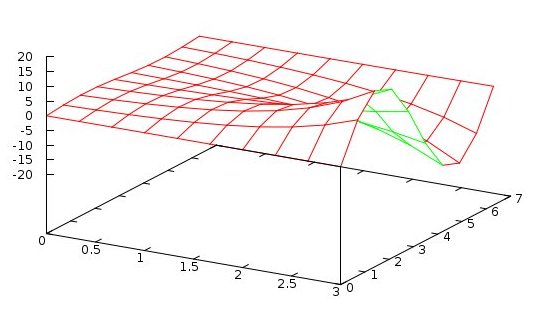
A simple PDE
Uxxxx(x,y,z,t) + Uyyyy(x,y,z,t) + Uzzzz(x,y,z,t) + Utttt(x,y,z,t) =
2*(exp(x)+exp(y)+exp(z)+exp(t))
with solution
U(x,y,z,t) = exp(x)+exp(y)+exp(z)+exp(t)
is shown below.
It runs very fast, yet accuracy problems as number of unknown
vertices increases.
This is very sensitive to the independence of the underlying
grid points.
nuderiv4d.java basic discretization
test_nuderiv4d.java test discretization
pde44e_nuderiv4d.java PDE source code
pde44e_nuderiv4d_1_java.out PDE solution
A third degree PDE over the more linearly independent 4D grid points
shows the error degradation with more free vertices.
The output has three accuracy tests, for 1, 5 and 10 free nodes.
pde34_nuderiv4d.java PDE source code
pde34_nuderiv4d_1_java.out PDE solution
non uniform distributed vertices in Ada
Basically same code as above, in Ada
nuderiv4d.ads basic discretization spec
nuderiv4d.adb basic discretization body
test_nuderiv4d.adb test discretization
test_nuderiv4d_ada.out test discretization output
pde44e_nuderiv4d.adb PDE source code
pde44e_nuderiv4d_ada.out PDE solution, output
An extended example of discretization of a fourth order PDE in two
non uniform dimensions is shown in discrete2d.txt
Error increases with higher derivative and fewer points
The minimum number of points to compute a derivative of order n is n+1.
More points used decreases the error until numeric failure.
e.g. without multiple precision, third and fourth order derivative
fail with 11 points. An example of the variation of error from
computing the derivative on a sine wave is shown by
test_deriv.c source to test
deriv.c basic discretization, uniform spacing
test_deriv_c.out output showing test
Just general test, Python2 py and Python3 py3
deriv.py basic discretization, uniform spacing
test_deriv.py source to test
test_deriv_py.out output showing test
test_deriv.py3 source to test
test_deriv_py3.out output showing test
rderiv.py just deriv uniform spacing
test_rderiv.py source to test
test_rderiv_py.out output showing test
test_rderiv.py3 source to test
test_rderiv_py3.out output showing test
nuderiv.py just deriv, non uniform spacing
test_nuderiv.py source to test
test_nuderiv_py.out output showing test
More testing in ruby
Inverse.rb Inverse class
Deriv.rb Deriv class
test_deriv.prb source to test
test_deriv_rb.out output showing test
Non uniform discretization follows the same error pattern and the maximum
error goes approximately as the largest spacing between points.
<- previous index next ->
-
CMSC 455 home page
-
Syllabus - class dates and subjects, homework dates, reading assignments
-
Homework assignments - the details
-
Projects -
-
Partial Lecture Notes, one per WEB page
-
Partial Lecture Notes, one big page for printing
-
Downloadable samples, source and executables
-
Some brief notes on Matlab
-
Some brief notes on Python
-
Some brief notes on Fortran 95
-
Some brief notes on Ada 95
-
An Ada math library (gnatmath95)
-
Finite difference approximations for derivatives
-
MATLAB examples, some ODE, some PDE
-
parallel threads examples
-
Reference pages on Taylor series, identities,
coordinate systems, differential operators
-
selected news related to numerical computation