<- previous index next ->
We now extend the analysis and solution to three dimensions and
unequal step sizes.
We are told there is an unknown function u(x,y,z) that satisfies
the partial differential equation:
(read 'd' as the partial derivative symbol, '^' as exponent)
d^2u(x,y,z)/dx^2 + d^2u(x,y,z)/dy^2 + d^2u(x,y,z)/dz^2 = c(x,y,z)
and we are given the function c(x,y,z)
and we are given the values of u(x,y,z) on the boundary
of the domain of x,y,z in xmin,ymin,zmin to xmax,ymax,zmax
To compute the numerical solution of u(x,y,z) at a set of points
we choose the number of points in the x,y and z directions, nx,ny,nz.
The number of non boundary points is called the degrees of freedom, DOF.
Thus we have a grid of cells typically programmed as a
three dimensional array.
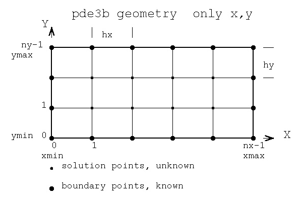 From the above we get a step size hx = (xmax-xmin)/(nx-1) ,
hy = (ymax-ymin)/(ny-1) and hz = (zmax-zmin)/(nz-1).
If we need u(x,y,z) at some point not on our solution grid,
we can use three dimensional interpolation to find the desired value.
Now, write the differential equation as a second order
numerical difference equation. The analytic derivatives are
made discrete by numerical approximation. "Discretization."
(Numerical derivatives from nderiv.out order 2, points 3, term 1)
d^2u(x,y,z)/dx^2 + d^2u(x,y,z)/dy^2 + d^2u(x,y,z)/d^2z =
1/h^2(u(x-h,y,z)-2u(x,y,z)+u(x+h,y,z)) +
1/h^2(u(x,y-h,z)-2u(x,y,z)+u(x,y+h,z)) +
1/h^2(u(x,y,z-h)-2u(x,y,z)+u(x,y,z+h)) + O(h^2)
Setting the above equal to c(x,y,z)
d^2u(x,y,z)/dx^2 + d^2u(x,y,z)/dy^2 + d^2u(x,y,z)/d^2z = c(x,y,z) becomes
1/hx^2(u(x-hx,y,z)+u(x+hx,y,z)-2u(x,y,z)) +
1/hy^2(u(x,y-hy,z)+u(x,y+hy,z)-2u(x,y,z)) +
1/hz^2(u(x,y,z-hz)+u(x,y,z+hz)-2u(x,y,z)) = c(x,y,z)
now solve for new u(x,y,z), based on neighboring grid points
u(x,y,z) = ((u(x-hx,y,z)+u(x+hx,y,z))/hx^2 +
(u(x,y-hy,z)+u(x,y+hy,z))/hy^2 +
(u(x,y,z-hz)+u(x,y,z+hz))/hz^2 - c(x,y,z)) /
(2/hx^2 + 2/hy^2 + 2/hz^2)
The formula for u(x,y,z) is programmed based on indexes i,j,k
such that x=xmin+i*hx, y=ymin+j*hy, z=zmin+k*hz
for i=1,nx-2 j=1,ny-2 k=1,nz-2
Note that the boundary values are set and unchanged for the six
sides i=0 for j=0,ny-1 k=0,nz-1 i=nx-1 for j=0,ny-1 k=0,nz-1
j=0 for i=0,nx-1 k=0,nz-1 j=ny-1 for i=0,nx-1 k=0,nz-1
k=0 for i=0,nx-1 j=0,nx-1 k=nz-1 for i=0,nx-1 j=0,ny-1
and the interior cells are set to some value, typically zero.
Then iterate, computing new interior cells based on the previous
set of cells including the boundary.
Compute the absolute value of the difference between each new
interior cell and the previous interior cell. A stable problem
will result in this value getting monotonically smaller.
The stopping condition may be based on the above difference
value or on the number of iterations.
To demonstrate the above development, a known u(x,y,z) is used.
The boundary values are set and the iterations computed.
Since the solution is known, the error can be computed at
each cell and reported for each iteration.
At several iterations, the computed solution and the errors
from the known exact solution are printed.
The same code has been programmed in "C", Java, Fortran 95 and Ada 95
as shown below with file types .c, .java, .f90 and .adb:
"C" source code pde3b.c
output of pde3b.c
Fortran 95 source code pde3b.f90
output of pde3b.f90
Java source code pde3b.java
output of pde3b.java
Ada 95 source code pde3b.adb
output of pde3b.adb
Matlab 7 source code pde3b.m
output of pde3b.m
It should be noted that a direct solution is possible.
The iterative solution comes from a large set of simultaneous
equations that may be able to be solved accurately. For the
same three dimensional problem above, observe the development
of the set of simultaneous equations:
We are told there is an unknown function u(x,y,z) that satisfies
the partial differential equation:
(read 'd' as the partial derivative symbol, '^' as exponent)
d^2u(x,y,z)/dx^2 + d^2u(x,y,z)/dy^2 + d^2u(x,y,z)/dz^2 = c(x,y,z)
and we are given the function c(x,y,z)
and we are given the values of u(x,y,z) on the boundary ub(x,y,z)
of the domain of x,y,z in xmin,ymin,zmin to xmax,ymax,zmax
To compute the numerical solution of u(x,y,z) at a set of points
we choose the number of points in the x,y and z directions, nx,ny,nz.
Thus we have a grid of cells typically programmed as a
three dimensional array.
From the above we get a step size hx = (xmax-ymin)/(nx-1) ,
hy = (ymax-ymin)/(ny-1) and hz = (xmax-zmin)/(nz-1).
If we need u(x,y,z) at some point not on our solution grid,
we can use three dimensional interpolation to find the desired value.
Now, write the differential equation as a second order
numerical difference equation.
(Numerical derivatives from nderiv.out order 2, points 3, term 1)
d^2u(x,y,z)/dx^2 + d^2u(x,y,z)/dy^2 + d^2u(x,y,z)/d^2z =
1/h^2(u(x-h,y,z)-2u(x,y,z)+u(x+h,y,z)) +
1/h^2(u(x,y-h,z)-2u(x,y,z)+u(x,y+h,z)) +
1/h^2(u(x,y,z-h)-2u(x,y,z)+u(x,y,z+h)) + O(h^2)
Setting the above equal to c(x,y,z)
d^2u(x,y,z)/dx^2 + d^2u(x,y,z)/dy^2 + d^2u(x,y,z)/d^2z = c(x,y,z) becomes
1/hx^2(u(x-hx,y,z)+u(x+hx,y,z)-2u(x,y,z)) +
1/hy^2(u(x,y-hy,z)+u(x,y+hy,z)-2u(x,y,z)) +
1/hz^2(u(x,y,z-hz)+u(x,y,z+hz)-2u(x,y,z)) = c(x,y,z)
Now, rearrange terms to collect the u(x,y,z) coefficients:
u(x-hx,y,z)/hx^2 + u(x+hx,y,z)/hx^2 +
u(x,y-hy,z)/hy^2 + u(x,y+hy,z)/hy^2 +
u(x,y,z-hz)/hz^2 + u(x,y,z+hz)/hz^2 -
u(x,y,z)*(2/hx^2 + 2/hy^2 + 2/hz^2) = c(x,y,z)
We build a linear system of simultaneous equations M U = V
by computing the values of the matrix M and right hand side vector V.
(The system of equations is linear if the differential equation is linear,
otherwise a system of nonlinear equations must be solved.)
The linear subscripts of U corresponding to u(i,j,k) is
m = (i-1)*(ny-2)*(nz-2) + (j-1)*(nz-2) + k
and the rows and columns and V use the same linear subscripts.
Now, using indexes rather than x, x+hx, x-hx,
solve system of linear equations for u(i,j,k).
u(i,j,k)=u(xmin+i*hx, ymin+j*hz, zmin+k*hz)
u(i-1,j,k)/hx^2 + u(i+1,j,k)/hx^2 +
u(i,j-1,k)/hy^2 + u(i,j+1,k)/hy^2 +
u(i,j,k-1)/hz^2 + u(i,j,k+1)/hz^2 -
u(i,j,k)*(2/hx^2 + 2/hy^2 + 2/hz^2) = c(x,y,z)
for i=1,nx-2 j=1,ny-2 k=1,nz-2 while substituting
u(i,j,k) boundary values when i=0 or nx-1, j=0 or ny-1,
k=0 or nz-1 using x=xmin+i*hx, y=ymin+j*hz, z=zmin+k*hz
Remember: hx, hy, hz are known constants, c(x,y,z) is computable.
The matrix has m = (nx-2)*(ny-2)*(nz-2) rows and columns for
solving for m equations in m unknowns. The right hand side vector
is the c(x,y,z) values with possibly boundary terms subtracted.
The unknowns are u(i,j,k) for i=1,nx-2, j=1,ny-2, k=1,nz-2 .
The first row of the matrix is for the unknown u(1,1,1) i=1, j=1, k=1
ub(xmin+0*hx,ymin+1*hy,zmin+1*hz)/hx^2 + u(2,1,1)/hx^2 +
ub(xmin+1*hx,ymin+0*hy,zmin+1*hz)/hy^2 + u(1,2,1)/hy^2 +
ub(xmin+1*hx,ymin+1*hy,zmin+0*hz)/hz^2 + u(1,1,2)/hz^2 +
u(1,1,1)*(2/hx^2 + 2/hy^2 + 2/hz^2) = c(xmin+1*hx,ymin+1*hy,zmin+1*hz)
Matrix cells in first row are zero except for:
M(1,1,1)(1,1,1) = 1/(2/hx^2 + 2/hy^2 + 2/hz^2)
M(1,1,1)(1,1,2) = 1/hz^2
M(1,1,1)(1,2,1) = 1/hy^2
M(1,1,1)(2,1,1) = 1/hx^2
V(1,1,1) = c(xmin+1*hx,ymin+1*hy,zmin+1*hz)
-ub(xmin+0*hx,ymin+1*hy,zmin+1*hz)/hx^2
-ub(xmin+1*hx,ymin+0*hy,zmin+1*hz)/hy^2
-ub(xmin+1*hx,ymin+1*hy,zmin+0*hz)/hz^2
Note that three of the terms are boundary terms and thus have a
computed value that is subtracted from the right hand side vector V.
The row of the matrix for the u(2,2,2) unknown has no boundary terms
u(1,2,2)/hx^2 + u(3,2,2)/hx^2 +
u(2,1,2)/hy^2 + u(2,3,2)/hy^2 +
u(2,2,1)/hz^2 + u(2,2,3)/hz^2 +
u(2,2,2)*(2/hx^2 + 2/hy^2 + 2/hz^2) = c(xmin+2*hx,ymin+2*hy,zmin+2*hz)
Matrix cells in row (2,2,2) are zero except for:
M(2,2,2)(1,2,2) = 1/hx^2
M(2,2,2)(3,2,2) = 1/hx^2
M(2,2,2)(2,1,2) = 1/hy^2
M(2,2,2)(2,3,2) = 1/hy^2
M(2,2,2)(2,2,1) = 1/hz^2
M(2,2,2)(2,2,3) = 1/hz^2
M(2,2,2)(2,2,2) = 1/(2/hx^2 + 2/hy^2 + 2/hz^2)
V(2,2,2) = c(xmin+2*hx,ymin+2*hy,zmin+2*hz)
The number of rows in the matrix is equal to the number of
equations to solve simultaneously and is equal to the
number of unknowns, the degrees of freedom.
The matrix is quite sparse and may be considered "band diagonal".
Typically, special purpose simultaneous equation solvers are
used, often with preconditioners.
A PDE that has all constant coefficients, in this case,
there are only four possible values in the matrix. These are
computed only once at the start of building the matrix.
A PDE with functions of x,y,z as coefficients is covered later.
Solving the system of equations for our test problem gave
the error on the order of 10^-12 compared with
the iterative solution error of 10^-4 after 150 iterations.
The same code has been programmed in "C", Java, Fortran 95, Ada 95 and
Matlab 7 as shown below with file types .c, .java, .f90, .adb and .m:
"C" source code pde3b_eq.c
output of pde3b_eq.c
Fortran 95 source code pde3b_eq.f90
output of pde3b_eq.f90
Java source code pde3b_eq.java
output of pde3b_eq.java
Ada 95 source code pde3b_eq.adb
output of pde3b_eq.adb
Matlab 7 source code pde3b_eq.m
output of pde3b_eq.m
Please note that the solution of partial differential equations
gets significantly more complicated if the solution is not
continuous or is not continuously differentiable.
You can tailor the code presented above for many second order partial
differential equations in three independent variables.
1) You must provide a function u(x,y,z) that computes the solution
on the boundaries. It does not have to be a complete solution and
the "check" code should be removed.
2) You must provide a function c(x,y,z) that computes the
forcing function, the right hand side of the differential equation.
3a) If the differential equation is not d^2/dx^2 + d^2/dy^2 +d^2/dz^2
then use coefficients from nderiv.out to create a new function
u000(i,j,k) that computes a new value of the solution at i,j,k
from the neighboring coordinates for the next iteration.
3b) If the differential equation is not d^2/dx^2 + d^2/dy^2 +d^2/dz^2
then use coefficients from nderiv.out to create a new matrix
initialization function and then solve the simultaneous equations.
3c) There may be constant or function multipliers in the given PDE.
For example exp(x+y/2) * d^2/dx^2 + 7 * d^2/dy^2 etc.
Constant multipliers are just multiplied when creating the
discrete equations. Functions of the independent variables, x,y
must be evaluated at the point where the discrete derivative is
being applied.
For an extended example of discretization of a fourth order PDE
in two dimensions see discrete2d.txt
Source code is available to compute coefficients for derivatives
of many orders. The source code is available in many languages,
deriv.h gives a good overview:
/* deriv.h compute formulas for numerical derivatives */
/* returns npoints values in a or c */
/* 0 <= point < npoints */
void deriv(int order, int npoints, int point, int *a, int *bb);
/* c[point][] = (1.0/((double)bb*h^order))*a[] */
void rderiv(int order, int npoints, int point, double h, double c[]);
/* c includes bb and h^order */
/* derivative of f(x) = c[0]*f(x+(0-point)*h) + */
/* c[1]*f(x+(1-point)*h) + */
/* c[2]*f(x+(2-point)*h) + ... + */
/* c[npoints-1]*f(x+(npoints-1-point)*h */
/* */
/* nuderiv give x values, not uniformly spaced, rather than h */
void nuderiv(int order, int npoints, int point, double x[], double c[]);
deriv.h
deriv.c
deriv.py
deriv.f90
Deriv.scala
deriv.adb
nuderiv.java non uniform, most general
Then the building of the simultaneous equations becomes:
double xg[] = {-1.0, -0.9, -0.8, -0.6, -0.3, 0.0,
0.35, 0.65, 0.85, 1.0, 1.2};
double cxx[] = new double[11]; // nuderiv coefficients
// coefdxx * d^2 u(x,y)/dx^2 for row ii in A matrix
coefdxx = 1.0; // could be a function of xg[i]
new nuderiv(2,nx,i,xg,cxx); // derivative coefficients
for(j=0; j<nx; j++) // cs is index of RHS
{
if(j==0 || j==nx-1)
A[ii][cs] = A[ii][cs] - coefdxx*cxx[j]*ubound(xg[j]);
else A[ii][j] = A[ii][j] + coefdxx*cxx[j];
}
extracted and modified from
pdenu22_eq.java
From the above we get a step size hx = (xmax-xmin)/(nx-1) ,
hy = (ymax-ymin)/(ny-1) and hz = (zmax-zmin)/(nz-1).
If we need u(x,y,z) at some point not on our solution grid,
we can use three dimensional interpolation to find the desired value.
Now, write the differential equation as a second order
numerical difference equation. The analytic derivatives are
made discrete by numerical approximation. "Discretization."
(Numerical derivatives from nderiv.out order 2, points 3, term 1)
d^2u(x,y,z)/dx^2 + d^2u(x,y,z)/dy^2 + d^2u(x,y,z)/d^2z =
1/h^2(u(x-h,y,z)-2u(x,y,z)+u(x+h,y,z)) +
1/h^2(u(x,y-h,z)-2u(x,y,z)+u(x,y+h,z)) +
1/h^2(u(x,y,z-h)-2u(x,y,z)+u(x,y,z+h)) + O(h^2)
Setting the above equal to c(x,y,z)
d^2u(x,y,z)/dx^2 + d^2u(x,y,z)/dy^2 + d^2u(x,y,z)/d^2z = c(x,y,z) becomes
1/hx^2(u(x-hx,y,z)+u(x+hx,y,z)-2u(x,y,z)) +
1/hy^2(u(x,y-hy,z)+u(x,y+hy,z)-2u(x,y,z)) +
1/hz^2(u(x,y,z-hz)+u(x,y,z+hz)-2u(x,y,z)) = c(x,y,z)
now solve for new u(x,y,z), based on neighboring grid points
u(x,y,z) = ((u(x-hx,y,z)+u(x+hx,y,z))/hx^2 +
(u(x,y-hy,z)+u(x,y+hy,z))/hy^2 +
(u(x,y,z-hz)+u(x,y,z+hz))/hz^2 - c(x,y,z)) /
(2/hx^2 + 2/hy^2 + 2/hz^2)
The formula for u(x,y,z) is programmed based on indexes i,j,k
such that x=xmin+i*hx, y=ymin+j*hy, z=zmin+k*hz
for i=1,nx-2 j=1,ny-2 k=1,nz-2
Note that the boundary values are set and unchanged for the six
sides i=0 for j=0,ny-1 k=0,nz-1 i=nx-1 for j=0,ny-1 k=0,nz-1
j=0 for i=0,nx-1 k=0,nz-1 j=ny-1 for i=0,nx-1 k=0,nz-1
k=0 for i=0,nx-1 j=0,nx-1 k=nz-1 for i=0,nx-1 j=0,ny-1
and the interior cells are set to some value, typically zero.
Then iterate, computing new interior cells based on the previous
set of cells including the boundary.
Compute the absolute value of the difference between each new
interior cell and the previous interior cell. A stable problem
will result in this value getting monotonically smaller.
The stopping condition may be based on the above difference
value or on the number of iterations.
To demonstrate the above development, a known u(x,y,z) is used.
The boundary values are set and the iterations computed.
Since the solution is known, the error can be computed at
each cell and reported for each iteration.
At several iterations, the computed solution and the errors
from the known exact solution are printed.
The same code has been programmed in "C", Java, Fortran 95 and Ada 95
as shown below with file types .c, .java, .f90 and .adb:
"C" source code pde3b.c
output of pde3b.c
Fortran 95 source code pde3b.f90
output of pde3b.f90
Java source code pde3b.java
output of pde3b.java
Ada 95 source code pde3b.adb
output of pde3b.adb
Matlab 7 source code pde3b.m
output of pde3b.m
It should be noted that a direct solution is possible.
The iterative solution comes from a large set of simultaneous
equations that may be able to be solved accurately. For the
same three dimensional problem above, observe the development
of the set of simultaneous equations:
We are told there is an unknown function u(x,y,z) that satisfies
the partial differential equation:
(read 'd' as the partial derivative symbol, '^' as exponent)
d^2u(x,y,z)/dx^2 + d^2u(x,y,z)/dy^2 + d^2u(x,y,z)/dz^2 = c(x,y,z)
and we are given the function c(x,y,z)
and we are given the values of u(x,y,z) on the boundary ub(x,y,z)
of the domain of x,y,z in xmin,ymin,zmin to xmax,ymax,zmax
To compute the numerical solution of u(x,y,z) at a set of points
we choose the number of points in the x,y and z directions, nx,ny,nz.
Thus we have a grid of cells typically programmed as a
three dimensional array.
From the above we get a step size hx = (xmax-ymin)/(nx-1) ,
hy = (ymax-ymin)/(ny-1) and hz = (xmax-zmin)/(nz-1).
If we need u(x,y,z) at some point not on our solution grid,
we can use three dimensional interpolation to find the desired value.
Now, write the differential equation as a second order
numerical difference equation.
(Numerical derivatives from nderiv.out order 2, points 3, term 1)
d^2u(x,y,z)/dx^2 + d^2u(x,y,z)/dy^2 + d^2u(x,y,z)/d^2z =
1/h^2(u(x-h,y,z)-2u(x,y,z)+u(x+h,y,z)) +
1/h^2(u(x,y-h,z)-2u(x,y,z)+u(x,y+h,z)) +
1/h^2(u(x,y,z-h)-2u(x,y,z)+u(x,y,z+h)) + O(h^2)
Setting the above equal to c(x,y,z)
d^2u(x,y,z)/dx^2 + d^2u(x,y,z)/dy^2 + d^2u(x,y,z)/d^2z = c(x,y,z) becomes
1/hx^2(u(x-hx,y,z)+u(x+hx,y,z)-2u(x,y,z)) +
1/hy^2(u(x,y-hy,z)+u(x,y+hy,z)-2u(x,y,z)) +
1/hz^2(u(x,y,z-hz)+u(x,y,z+hz)-2u(x,y,z)) = c(x,y,z)
Now, rearrange terms to collect the u(x,y,z) coefficients:
u(x-hx,y,z)/hx^2 + u(x+hx,y,z)/hx^2 +
u(x,y-hy,z)/hy^2 + u(x,y+hy,z)/hy^2 +
u(x,y,z-hz)/hz^2 + u(x,y,z+hz)/hz^2 -
u(x,y,z)*(2/hx^2 + 2/hy^2 + 2/hz^2) = c(x,y,z)
We build a linear system of simultaneous equations M U = V
by computing the values of the matrix M and right hand side vector V.
(The system of equations is linear if the differential equation is linear,
otherwise a system of nonlinear equations must be solved.)
The linear subscripts of U corresponding to u(i,j,k) is
m = (i-1)*(ny-2)*(nz-2) + (j-1)*(nz-2) + k
and the rows and columns and V use the same linear subscripts.
Now, using indexes rather than x, x+hx, x-hx,
solve system of linear equations for u(i,j,k).
u(i,j,k)=u(xmin+i*hx, ymin+j*hz, zmin+k*hz)
u(i-1,j,k)/hx^2 + u(i+1,j,k)/hx^2 +
u(i,j-1,k)/hy^2 + u(i,j+1,k)/hy^2 +
u(i,j,k-1)/hz^2 + u(i,j,k+1)/hz^2 -
u(i,j,k)*(2/hx^2 + 2/hy^2 + 2/hz^2) = c(x,y,z)
for i=1,nx-2 j=1,ny-2 k=1,nz-2 while substituting
u(i,j,k) boundary values when i=0 or nx-1, j=0 or ny-1,
k=0 or nz-1 using x=xmin+i*hx, y=ymin+j*hz, z=zmin+k*hz
Remember: hx, hy, hz are known constants, c(x,y,z) is computable.
The matrix has m = (nx-2)*(ny-2)*(nz-2) rows and columns for
solving for m equations in m unknowns. The right hand side vector
is the c(x,y,z) values with possibly boundary terms subtracted.
The unknowns are u(i,j,k) for i=1,nx-2, j=1,ny-2, k=1,nz-2 .
The first row of the matrix is for the unknown u(1,1,1) i=1, j=1, k=1
ub(xmin+0*hx,ymin+1*hy,zmin+1*hz)/hx^2 + u(2,1,1)/hx^2 +
ub(xmin+1*hx,ymin+0*hy,zmin+1*hz)/hy^2 + u(1,2,1)/hy^2 +
ub(xmin+1*hx,ymin+1*hy,zmin+0*hz)/hz^2 + u(1,1,2)/hz^2 +
u(1,1,1)*(2/hx^2 + 2/hy^2 + 2/hz^2) = c(xmin+1*hx,ymin+1*hy,zmin+1*hz)
Matrix cells in first row are zero except for:
M(1,1,1)(1,1,1) = 1/(2/hx^2 + 2/hy^2 + 2/hz^2)
M(1,1,1)(1,1,2) = 1/hz^2
M(1,1,1)(1,2,1) = 1/hy^2
M(1,1,1)(2,1,1) = 1/hx^2
V(1,1,1) = c(xmin+1*hx,ymin+1*hy,zmin+1*hz)
-ub(xmin+0*hx,ymin+1*hy,zmin+1*hz)/hx^2
-ub(xmin+1*hx,ymin+0*hy,zmin+1*hz)/hy^2
-ub(xmin+1*hx,ymin+1*hy,zmin+0*hz)/hz^2
Note that three of the terms are boundary terms and thus have a
computed value that is subtracted from the right hand side vector V.
The row of the matrix for the u(2,2,2) unknown has no boundary terms
u(1,2,2)/hx^2 + u(3,2,2)/hx^2 +
u(2,1,2)/hy^2 + u(2,3,2)/hy^2 +
u(2,2,1)/hz^2 + u(2,2,3)/hz^2 +
u(2,2,2)*(2/hx^2 + 2/hy^2 + 2/hz^2) = c(xmin+2*hx,ymin+2*hy,zmin+2*hz)
Matrix cells in row (2,2,2) are zero except for:
M(2,2,2)(1,2,2) = 1/hx^2
M(2,2,2)(3,2,2) = 1/hx^2
M(2,2,2)(2,1,2) = 1/hy^2
M(2,2,2)(2,3,2) = 1/hy^2
M(2,2,2)(2,2,1) = 1/hz^2
M(2,2,2)(2,2,3) = 1/hz^2
M(2,2,2)(2,2,2) = 1/(2/hx^2 + 2/hy^2 + 2/hz^2)
V(2,2,2) = c(xmin+2*hx,ymin+2*hy,zmin+2*hz)
The number of rows in the matrix is equal to the number of
equations to solve simultaneously and is equal to the
number of unknowns, the degrees of freedom.
The matrix is quite sparse and may be considered "band diagonal".
Typically, special purpose simultaneous equation solvers are
used, often with preconditioners.
A PDE that has all constant coefficients, in this case,
there are only four possible values in the matrix. These are
computed only once at the start of building the matrix.
A PDE with functions of x,y,z as coefficients is covered later.
Solving the system of equations for our test problem gave
the error on the order of 10^-12 compared with
the iterative solution error of 10^-4 after 150 iterations.
The same code has been programmed in "C", Java, Fortran 95, Ada 95 and
Matlab 7 as shown below with file types .c, .java, .f90, .adb and .m:
"C" source code pde3b_eq.c
output of pde3b_eq.c
Fortran 95 source code pde3b_eq.f90
output of pde3b_eq.f90
Java source code pde3b_eq.java
output of pde3b_eq.java
Ada 95 source code pde3b_eq.adb
output of pde3b_eq.adb
Matlab 7 source code pde3b_eq.m
output of pde3b_eq.m
Please note that the solution of partial differential equations
gets significantly more complicated if the solution is not
continuous or is not continuously differentiable.
You can tailor the code presented above for many second order partial
differential equations in three independent variables.
1) You must provide a function u(x,y,z) that computes the solution
on the boundaries. It does not have to be a complete solution and
the "check" code should be removed.
2) You must provide a function c(x,y,z) that computes the
forcing function, the right hand side of the differential equation.
3a) If the differential equation is not d^2/dx^2 + d^2/dy^2 +d^2/dz^2
then use coefficients from nderiv.out to create a new function
u000(i,j,k) that computes a new value of the solution at i,j,k
from the neighboring coordinates for the next iteration.
3b) If the differential equation is not d^2/dx^2 + d^2/dy^2 +d^2/dz^2
then use coefficients from nderiv.out to create a new matrix
initialization function and then solve the simultaneous equations.
3c) There may be constant or function multipliers in the given PDE.
For example exp(x+y/2) * d^2/dx^2 + 7 * d^2/dy^2 etc.
Constant multipliers are just multiplied when creating the
discrete equations. Functions of the independent variables, x,y
must be evaluated at the point where the discrete derivative is
being applied.
For an extended example of discretization of a fourth order PDE
in two dimensions see discrete2d.txt
Source code is available to compute coefficients for derivatives
of many orders. The source code is available in many languages,
deriv.h gives a good overview:
/* deriv.h compute formulas for numerical derivatives */
/* returns npoints values in a or c */
/* 0 <= point < npoints */
void deriv(int order, int npoints, int point, int *a, int *bb);
/* c[point][] = (1.0/((double)bb*h^order))*a[] */
void rderiv(int order, int npoints, int point, double h, double c[]);
/* c includes bb and h^order */
/* derivative of f(x) = c[0]*f(x+(0-point)*h) + */
/* c[1]*f(x+(1-point)*h) + */
/* c[2]*f(x+(2-point)*h) + ... + */
/* c[npoints-1]*f(x+(npoints-1-point)*h */
/* */
/* nuderiv give x values, not uniformly spaced, rather than h */
void nuderiv(int order, int npoints, int point, double x[], double c[]);
deriv.h
deriv.c
deriv.py
deriv.f90
Deriv.scala
deriv.adb
nuderiv.java non uniform, most general
Then the building of the simultaneous equations becomes:
double xg[] = {-1.0, -0.9, -0.8, -0.6, -0.3, 0.0,
0.35, 0.65, 0.85, 1.0, 1.2};
double cxx[] = new double[11]; // nuderiv coefficients
// coefdxx * d^2 u(x,y)/dx^2 for row ii in A matrix
coefdxx = 1.0; // could be a function of xg[i]
new nuderiv(2,nx,i,xg,cxx); // derivative coefficients
for(j=0; j<nx; j++) // cs is index of RHS
{
if(j==0 || j==nx-1)
A[ii][cs] = A[ii][cs] - coefdxx*cxx[j]*ubound(xg[j]);
else A[ii][j] = A[ii][j] + coefdxx*cxx[j];
}
extracted and modified from
pdenu22_eq.java
<- previous index next ->
-
CMSC 455 home page
-
Syllabus - class dates and subjects, homework dates, reading assignments
-
Homework assignments - the details
-
Projects -
-
Partial Lecture Notes, one per WEB page
-
Partial Lecture Notes, one big page for printing
-
Downloadable samples, source and executables
-
Some brief notes on Matlab
-
Some brief notes on Python
-
Some brief notes on Fortran 95
-
Some brief notes on Ada 95
-
An Ada math library (gnatmath95)
-
Finite difference approximations for derivatives
-
MATLAB examples, some ODE, some PDE
-
parallel threads examples
-
Reference pages on Taylor series, identities,
coordinate systems, differential operators
-
selected news related to numerical computation