<- previous index next ->
Some partial differential equations are difficult to solve symbolically
and some are difficult to solve numerically.
This lecture covers the numerical solution of simple partial
differential equations where the boundary values are known.
See simple definitions .
We are told there is an unknown function u(x,y) that satisfies
the partial differential equation:
(read 'd' as the partial derivative symbol, '^' as exponent)
d^2u(x,y)/dx^2 + d^2u(x,y)/dy^2 = c(x,y)
and we are given the function c(x,y)
and we are given the values of u(x,y) on the boundary
of the domain of x,y in xmin,ymin to xmax,ymax
To compute the numerical solution of u(x,y) at a set of points
we choose the number of points in the x and y directions, nx, ny.
Thus we have a grid of cells typically programmed as a
two dimensional array.
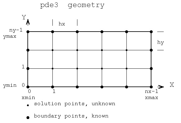 The number of solution points, unknowns, is typically called
the degrees of freedom, DOF.
From the above we get a step size hx = (xmax-xmin)/(nx-1) and
hy = (ymax-ymin)/(ny-1). For our first solution we choose
hx = hy = h and just use a step size of h.
If we need u(x,y) at some point not on our solution grid,
we can use two dimensional interpolation to find the desired value.
Now, write the differential equation as a second order
numerical difference equation.
(Numerical derivatives from nderiv.out order 2, points 3, term 1)
d^2u(x,y)/dx^2 + d^2u(x,y)/dy^2 =
1/h^2(u(x-h,y)-2u(x,y)+u(x+h,y)) +
1/h^2(u(x,y-h)-2u(x,y)+u(x,y+h)) +O(h^2)
Setting the above equal to c(x,y) and collecting terms
d^2u(x,y)/dx^2 + d^2u(x,y)/dy^2 = c(x,y) becomes
1/h^2(u(x-h,y)+u(x+h,y)+u(x,y-h)+u(x,y+h)-4u(x,y))=c(x,y)
now solve for a new u(x,y), based on neighboring grid points
u(x,y)= (u(x-h,y)+u(x+h,0)+u(x,y-h)+u(x,y+h)-c(x,y)*h^2)/4
The formula for u(x,y) is programmed based on indexes i and j
such that x=xmin+i*h, y=ymin+j*h for i=1,nx-2 j=1,ny-2
Note that the boundary values are set and unchanged for the four
sides i=0 for j=0,ny-1 i=nx-1 for j=0,ny-1
j=0 for i=0,nx-1 j=ny-1 for i=0,nx-1
and the interior cells are set to some value, typically zero.
Then iterate, computing new interior cells based on the previous
set of cells including the boundary.
Compute the absolute value of the difference between each new
interior cell and the previous interior cell. A stable problem
will result in this value getting monotonically smaller.
The stopping condition may be based on the above difference
value or on the number of iterations.
To demonstrate the above development, a known u(x,y) is used.
The boundary values are set and the iterations computed.
Since the solution is known, the error can be computed at
each cell and reported for each iteration.
At several iterations, the computed solution and the errors
from the known exact solution are printed.
The same code has been programmed in "C", Java, Fortran 95, Ada 95 and
Matlab as shown below with file types .c, .java, .f90, .adb and .m:
Chose the language you like best and get an understanding of
how the method above was programmed.
"C" source code pde3.c
output of pde3.c
Fortran 95 source code pde3.f90
output of pde3.f90
Java source code pde3.java
output of pde3.java
Ada 95 source code pde3.adb
output of pde3.adb
Matlab 7 source code pde3.m
output of pde3.m
You may tailor any of the above code to solve second order
partial differential equations in two independent variables.
1) You need a function c(x,y) that is the forcing function, the right
hand side of the differential equation.
2) You need a function u(x,y) that provides at least the boundary
conditions. If your u(x,y) is not a test solution, remove the "check"
code. And a choice of xmin, xmax, ymin, ymax.
3) If your differential equation is different, then use nderiv.out
to find the coefficients and create the function u00(i,j) that
computes the next value of a solution point from the surrounding
previous solution points.
The following examples will be covered for a more general case
in the next lecture. The same problem is solved as given above,
using a method of solving simultaneous linear equations, rather
than an iterative method. The files corresponding to the above
examples are with minimum modifications are:
derivation of pde3_eq.c
"C" source code pde3_eq.c
output of pde3_eq.c
Matlab 7 source code pde3_eq.m
output of pde3_eq.m
The number of solution points, unknowns, is typically called
the degrees of freedom, DOF.
From the above we get a step size hx = (xmax-xmin)/(nx-1) and
hy = (ymax-ymin)/(ny-1). For our first solution we choose
hx = hy = h and just use a step size of h.
If we need u(x,y) at some point not on our solution grid,
we can use two dimensional interpolation to find the desired value.
Now, write the differential equation as a second order
numerical difference equation.
(Numerical derivatives from nderiv.out order 2, points 3, term 1)
d^2u(x,y)/dx^2 + d^2u(x,y)/dy^2 =
1/h^2(u(x-h,y)-2u(x,y)+u(x+h,y)) +
1/h^2(u(x,y-h)-2u(x,y)+u(x,y+h)) +O(h^2)
Setting the above equal to c(x,y) and collecting terms
d^2u(x,y)/dx^2 + d^2u(x,y)/dy^2 = c(x,y) becomes
1/h^2(u(x-h,y)+u(x+h,y)+u(x,y-h)+u(x,y+h)-4u(x,y))=c(x,y)
now solve for a new u(x,y), based on neighboring grid points
u(x,y)= (u(x-h,y)+u(x+h,0)+u(x,y-h)+u(x,y+h)-c(x,y)*h^2)/4
The formula for u(x,y) is programmed based on indexes i and j
such that x=xmin+i*h, y=ymin+j*h for i=1,nx-2 j=1,ny-2
Note that the boundary values are set and unchanged for the four
sides i=0 for j=0,ny-1 i=nx-1 for j=0,ny-1
j=0 for i=0,nx-1 j=ny-1 for i=0,nx-1
and the interior cells are set to some value, typically zero.
Then iterate, computing new interior cells based on the previous
set of cells including the boundary.
Compute the absolute value of the difference between each new
interior cell and the previous interior cell. A stable problem
will result in this value getting monotonically smaller.
The stopping condition may be based on the above difference
value or on the number of iterations.
To demonstrate the above development, a known u(x,y) is used.
The boundary values are set and the iterations computed.
Since the solution is known, the error can be computed at
each cell and reported for each iteration.
At several iterations, the computed solution and the errors
from the known exact solution are printed.
The same code has been programmed in "C", Java, Fortran 95, Ada 95 and
Matlab as shown below with file types .c, .java, .f90, .adb and .m:
Chose the language you like best and get an understanding of
how the method above was programmed.
"C" source code pde3.c
output of pde3.c
Fortran 95 source code pde3.f90
output of pde3.f90
Java source code pde3.java
output of pde3.java
Ada 95 source code pde3.adb
output of pde3.adb
Matlab 7 source code pde3.m
output of pde3.m
You may tailor any of the above code to solve second order
partial differential equations in two independent variables.
1) You need a function c(x,y) that is the forcing function, the right
hand side of the differential equation.
2) You need a function u(x,y) that provides at least the boundary
conditions. If your u(x,y) is not a test solution, remove the "check"
code. And a choice of xmin, xmax, ymin, ymax.
3) If your differential equation is different, then use nderiv.out
to find the coefficients and create the function u00(i,j) that
computes the next value of a solution point from the surrounding
previous solution points.
The following examples will be covered for a more general case
in the next lecture. The same problem is solved as given above,
using a method of solving simultaneous linear equations, rather
than an iterative method. The files corresponding to the above
examples are with minimum modifications are:
derivation of pde3_eq.c
"C" source code pde3_eq.c
output of pde3_eq.c
Matlab 7 source code pde3_eq.m
output of pde3_eq.m
Method using solution of simultaneous equations,
rather than an iterative method
Extending to four dimensions in four variables causes the
indexing to get more complex, yet the implementation is
still systematic. An example in C, Java, Ada and Fortran is:
Note that a fourth order method is used when the solution
is at most a fourth order polynomial, thus very small
errors are expected.
"C" source code pde44_eq.c
output is pde44_eq_c.out
"C" source code simeq.c
"C" source code simeq.h
"C" source code deriv.c
"C" source code deriv.h
"java" source code pde44_eq.java
output is pde44_eq_java.out
"java" source code simeq.java
"java" source code rderiv.java
"java" source code test_rderiv.java
output is test_rderiv_java.out
"Ada" source code pde44_eq.adb
output is pde44_eq_ada.out
"Ada" source code pde44h_eq.adb
output is pde44h_eq_ada.out
"Ada" source code simeq.adb
"Ada" source code rderiv.adb
"Ada" source code real_arrays.ads
"Ada" source code real_arrays.adb
"Fortran" source code pde44_eq.f90
output is pde44_eq_f90.out
"Fortran" source code simeq.f90
"Fortran" source code deriv.f90
"Scala" source code Pde44_eq.scala
output is Pde44_eq_scala.out
"Scala" source code Pde44h_eq.scala
output is Pde44h_eq_scala.out
"Scala" source code Simeq.scala
"Scala" source code Deriv.scala
Then, the same set using sparse matrix
"C" source code pde44_sparse.c
output is pde44_sparse_c.out
"C" source code sparse.c
"C" source code sparse.h
"C" source code deriv.c
"C" source code deriv.h
"java" source code pde44_sparse.java
output is pde44_sparse_java.out
"java" source code sparse.java
"java" source code rderiv.java
"Ada" source code pde44_sparse.adb
output is pde44_sparse_ada.out
"Ada" source code sparse1.ads
"Ada" source code sparse1.adb
"Ada" source code rderiv.adb
"Ada" source code real_arrays.ads
"Ada" source code real_arrays.adb
(be careful: sparse.ads is zero based subscript,
sparse1.ads is one based subscript)
The instructor understands that some students have a strong
prejudice in favor of, or against, some programming languages.
After about 50 years of programming in about 17 programming
languages, the instructor finds that the difference between
programming languages is mostly syntactic sugar. Yet, since
students may be able to read some programming languages
easier than others, these examples are presented in "C",
Fortran 90, Java, Ada and Matlab. The intent was to do a quick
translation, keeping most of the source code the same,
for the different languages. Style was not a consideration.
Some rearranging of the order was used when convenient.
In Java and Ada the quick and dirty formatting was used
and thus it is suggested to look at the formatted output of
"C" or Fortran. The numerical results are almost exactly
the same although the presentation differs considerably.
The Matlab code is a combination of "C" and Fortran given
as a single file with internal functions. The subscript base
is shifted from 0 to 1 as in Fortran.
All of this source code compiles and runs on Windows, Linux
and MacOSX. You should not care what operating system your
code will be executed on. Make it operating-system independent.
A very different method, FEM, Finite Element Method
Galerkin FEM overview
<- previous index next ->
-
CMSC 455 home page
-
Syllabus - class dates and subjects, homework dates, reading assignments
-
Homework assignments - the details
-
Projects -
-
Partial Lecture Notes, one per WEB page
-
Partial Lecture Notes, one big page for printing
-
Downloadable samples, source and executables
-
Some brief notes on Matlab
-
Some brief notes on Python
-
Some brief notes on Fortran 95
-
Some brief notes on Ada 95
-
An Ada math library (gnatmath95)
-
Finite difference approximations for derivatives
-
MATLAB examples, some ODE, some PDE
-
parallel threads examples
-
Reference pages on Taylor series, identities,
coordinate systems, differential operators
-
selected news related to numerical computation