<- previous index next ->
Quick and dirty numerical solution
Using the notation y for y(x), y' for d y(x)/dx, y'' for d^2 y(x)/dx^2 etc.
To solve a(x) y''' + b(x) y'' + c(x) y' + d(x) y + e(x) = 0
for y at one or more values of x,
with initial condition constants c1, c2, c3 at x0:
y(x0) = c1 y'(x0) = c2 y''(x0) = c3
Create a function that computes y''' =
f(ypp, yp, y, x) = -(b(x)*ypp + c(x)*yp + d(x)*y + e(x))/a(x)
(moving everything except y''' to right-hand-side of equation,
then divide by a(x) )
a(x), b(x), c(x), d(x) and e(x) may be any functions of x and
that includes constants and zero. a(x) must not equal zero in
the range of x0 .. desired largest x.
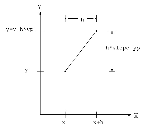 Diagram for y = y + h*yp moving from x to x+h
similarly yp = yp + h*ypp
similarly ypp = ypp + h*yppp
Initialize x = x0
y = c1
yp = c2
ypp = c3
loop: use some method with the function, f, to compute the next ypp
yppp=f(ypp, yp, y, x)
ypp = ypp + h*yppp first order or use some higher order
yp = yp + h*ypp or some higher order method
y = y + h*yp or some higher order method
x = x + h increment x and loop
optional, print y at this x
Quit when you have solved for y at the largest desired x
You may save previous values of x and y, interpolate at desired
value of x to get y.
You may run again with h half as big, keep halving h until you get
approximately the same result.
Quick and dirty finished! This actually works sometimes.
"x" is called the independent variable and
"y" is called the dependent variable.
This is known as an "initial value problem"
The conditions are known at the start and the definition of the
problem is used to numerically compute each successive value of
the solution. This was the method used to compute the flight
of the rocket in homework 1.
Later, we will cover a "boundary value problem" where at least
some information is given at the beginning and end of the
independent variable(s).
Diagram for y = y + h*yp moving from x to x+h
similarly yp = yp + h*ypp
similarly ypp = ypp + h*yppp
Initialize x = x0
y = c1
yp = c2
ypp = c3
loop: use some method with the function, f, to compute the next ypp
yppp=f(ypp, yp, y, x)
ypp = ypp + h*yppp first order or use some higher order
yp = yp + h*ypp or some higher order method
y = y + h*yp or some higher order method
x = x + h increment x and loop
optional, print y at this x
Quit when you have solved for y at the largest desired x
You may save previous values of x and y, interpolate at desired
value of x to get y.
You may run again with h half as big, keep halving h until you get
approximately the same result.
Quick and dirty finished! This actually works sometimes.
"x" is called the independent variable and
"y" is called the dependent variable.
This is known as an "initial value problem"
The conditions are known at the start and the definition of the
problem is used to numerically compute each successive value of
the solution. This was the method used to compute the flight
of the rocket in homework 1.
Later, we will cover a "boundary value problem" where at least
some information is given at the beginning and end of the
independent variable(s).
Better numerical solutions, Runge Kutta
To see some more accurate solutions to very simple ODE's
Solve y' = y y(0)=1 which is just y'(x) = y(x) = exp(x)
Initialize x = 0
y = 1
loop: use yp = y for exp low order method
y = y + h*y yp is just y
x = x + h increment x and loop
print y at this x
Initialize x = 0 Runge Kutta 4th order method
y = 1 this would be exact, within roundoff error,
if solution was 4th order or less polynomial
loop: use yp = y for exp fourth order method for y' = y y=exp(x)
k1 = h*y yp = f(x,y) in general
k2 = h*y+k1/2 f(x+h/2.0,y+k1/2.0)
k3 = h*y+k2/2 f(x+h/2.0,y+k2/2.0)
k4 = h*y+k3 f(x+h,y+k3)
y = y+(k1+2.0*k2+2.0*k3+k4)/6.0
x = x+h print y at this x
rk1_xy_acc.java using RK 4th order
rk1_xy_acc_java.out using RK 4th order
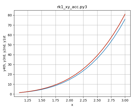
rk1_xy_acc.py3 using RK 4th order
rk1_xy_acc_py3.out using RK 4th order
 ode_exp.c using RK 4th order method
ode_exp_c.out note very small h is worse
To see some more accurate solutions to simple second order ODE's
Solve y'' = -y y(0)=1 y'(0)=0 which is just y(x)= cos(x)
ode_cos.c
ode_cos_c.out many cycles
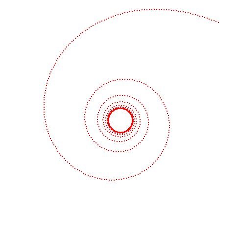
An example of an unstable ODE is Hopf:
p is a bifurcation parameter, constant for each solution.
Given: dx = gx(x,y,p) = p*x - y - x*(x^2+y^2)
dy = gy(x,y,p) = x + p*y - y*(x^2+y^2)
dr = sqrt(dx^2 + dy^2)
z = f(x,y,p)
Integrate from t=0 to t=tfinal
dz(x,y,p)/dt = dx/dr and
dz(x,y,p)/dt = dy/dr
The plot below uses initial conditions p=-0.1, x=0.4, y=0.4, t=0.0, dt=0.01
and runs to t=10.0
hopf_ode.c
ode_exp.c using RK 4th order method
ode_exp_c.out note very small h is worse
To see some more accurate solutions to simple second order ODE's
Solve y'' = -y y(0)=1 y'(0)=0 which is just y(x)= cos(x)
ode_cos.c
ode_cos_c.out many cycles
An example of an unstable ODE is Hopf:
p is a bifurcation parameter, constant for each solution.
Given: dx = gx(x,y,p) = p*x - y - x*(x^2+y^2)
dy = gy(x,y,p) = x + p*y - y*(x^2+y^2)
dr = sqrt(dx^2 + dy^2)
z = f(x,y,p)
Integrate from t=0 to t=tfinal
dz(x,y,p)/dt = dx/dr and
dz(x,y,p)/dt = dy/dr
The plot below uses initial conditions p=-0.1, x=0.4, y=0.4, t=0.0, dt=0.01
and runs to t=10.0
hopf_ode.c
 A three body problem, using simple integration, shows the
sling-shot effect of gravity when bodies get close.
Remember force of gravity F = G * mass1 * mass2 / distance^2
This is numerically very unstable.
body3.c needs OpenGL to compile and link.
Hopefully, it can be demonstrated running in class.
body3.java plain Java, different version.
Hopefully, it can be demonstrated running in class.
Center of Mass, Barycenter, general motion
For more typical ordinary differential equations there are some
classic methods. A common higher order method is Runge-Kutta fourth
order.
Given y' = f(x,y) and the initial values of x and y
L: k1 = h * f(x,y)
k2 = h * f(x+h/2.0,y+k1/2.0)
k3 = h * f(x+h/2.0,y+k2/2.0)
k4 = h * f(x+h,y+k3)
y = y + (k1+2.0*k2+2.0*k3+k4)/6.0
x = x + h
quit when x>your_biggest_x
loop to L:
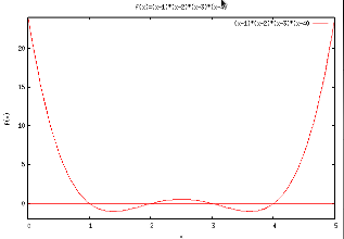
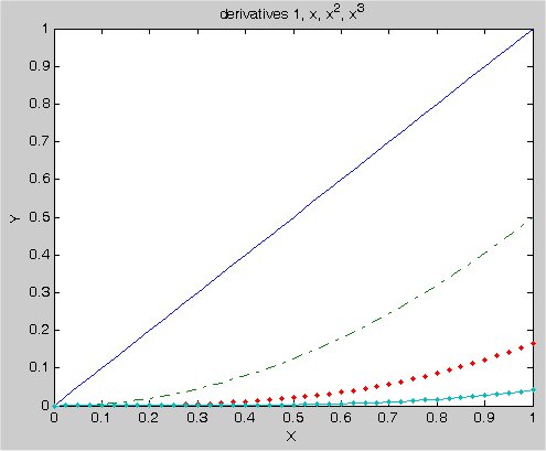
When the solution y(x) is a fourth order polynomial, or lower
order polynomial, the solution will be computed with no truncation
error, yet may have some roundoff error. Very large step sizes, h,
may be used for this very special case.
f(x)=(x-1)*(x-2)*(x-3)*(x-4) 4 roots, and =24 at x=0, x=5
A three body problem, using simple integration, shows the
sling-shot effect of gravity when bodies get close.
Remember force of gravity F = G * mass1 * mass2 / distance^2
This is numerically very unstable.
body3.c needs OpenGL to compile and link.
Hopefully, it can be demonstrated running in class.
body3.java plain Java, different version.
Hopefully, it can be demonstrated running in class.
Center of Mass, Barycenter, general motion
For more typical ordinary differential equations there are some
classic methods. A common higher order method is Runge-Kutta fourth
order.
Given y' = f(x,y) and the initial values of x and y
L: k1 = h * f(x,y)
k2 = h * f(x+h/2.0,y+k1/2.0)
k3 = h * f(x+h/2.0,y+k2/2.0)
k4 = h * f(x+h,y+k3)
y = y + (k1+2.0*k2+2.0*k3+k4)/6.0
x = x + h
quit when x>your_biggest_x
loop to L:
When the solution y(x) is a fourth order polynomial, or lower
order polynomial, the solution will be computed with no truncation
error, yet may have some roundoff error. Very large step sizes, h,
may be used for this very special case.
f(x)=(x-1)*(x-2)*(x-3)*(x-4) 4 roots, and =24 at x=0, x=5
 RK4th.java Java example
RK4th_java.out
RK4th.py Python example
RK4th_py.out
RK4th.rb Ruby example
RK4th_ruby.out
RK4th.java Scala example
RK4th_scala.out
In general, the solution will not be accurately approximated by
a low order polynomial. Thus, even the Runge-Kutta method may
require a very small step size in order to compute an accurate
solution. Because very small step sizes result in long computations
and may have large accumulations of roundoff error, variable
step size methods are often used.
Typically a maximum step size and a minimum step size are set.
Starting with some intermediate step size, h, the computation
proceeds as shown below.
Given y' = f(x,y) and the initial values of x and y
L: y1 = y + dy1 using some method with step size h compute dy1
the value of y1 is at x = x + h
y2a = y + dy2a using same method with step size h/2 compute dy2a
the value of y2a is at x = x + h/2
y2 = y2a + dy2 using same method, from y2a at x = x + h/2
with step size h/2 compute dy2
the value of y2 is at x = x + h
abs(y1-y2)>tolerance h = h/2, loop to L:
abs(y1-y2) < tolerance/4 h = 2 * h
y = y2
x = x + h
loop to L: until x > final x
There are many variations on the variable step size method.
The above is one simple version, partially demonstrated by:
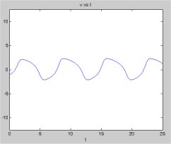
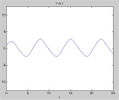
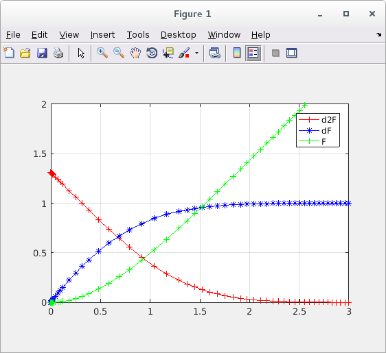
FitzHugh-Nagumo equations system of two ODE's
v' = v - v^3/3.0 + r initial v = -1.0
r' = -(v - 0.2 - 0.2*r) initial r = 1.0
initial h = 0.001
t in 0 .. 25
fitz.c just decreasing step size
fitz.out about equally spaced output
fitz.m easier to understand, MatLab
RK4th.java Java example
RK4th_java.out
RK4th.py Python example
RK4th_py.out
RK4th.rb Ruby example
RK4th_ruby.out
RK4th.java Scala example
RK4th_scala.out
In general, the solution will not be accurately approximated by
a low order polynomial. Thus, even the Runge-Kutta method may
require a very small step size in order to compute an accurate
solution. Because very small step sizes result in long computations
and may have large accumulations of roundoff error, variable
step size methods are often used.
Typically a maximum step size and a minimum step size are set.
Starting with some intermediate step size, h, the computation
proceeds as shown below.
Given y' = f(x,y) and the initial values of x and y
L: y1 = y + dy1 using some method with step size h compute dy1
the value of y1 is at x = x + h
y2a = y + dy2a using same method with step size h/2 compute dy2a
the value of y2a is at x = x + h/2
y2 = y2a + dy2 using same method, from y2a at x = x + h/2
with step size h/2 compute dy2
the value of y2 is at x = x + h
abs(y1-y2)>tolerance h = h/2, loop to L:
abs(y1-y2) < tolerance/4 h = 2 * h
y = y2
x = x + h
loop to L: until x > final x
There are many variations on the variable step size method.
The above is one simple version, partially demonstrated by:
FitzHugh-Nagumo equations system of two ODE's
v' = v - v^3/3.0 + r initial v = -1.0
r' = -(v - 0.2 - 0.2*r) initial r = 1.0
initial h = 0.001
t in 0 .. 25
fitz.c just decreasing step size
fitz.out about equally spaced output
fitz.m easier to understand, MatLab
 Of course, we can let MatLab solve the same ODE system
fitz2.m using MatLab ode45
The ode45 in MatLab uses a fourth order Runge-Kutta and then
a fifth order Runge-Kutta and compares the result. A neat formulation
is used to minimize the number of required function evaluations.
The fifth order method reuses some of the fourth order evaluations.
Written in "C" from p355 of textbook
fitz2.c similar to fitz.c
fitz2.out close to same results
A second order differential equation use or Runge-Kutta is demonstrated in:
rk4th_second.c
rk4th_second_c.out
A fourth order differential equation use or Runge-Kutta is demonstrated in:
rk4th_fourth.c
rk4th_fourth_c.out
rk4th_fourth.java
rk4th_fourth_java.out
Another coding of fourth order Runge-Kutta known as Gill's method
is the (subroutine, method, function) Runge given in a few languages.
The user provided code comes first, then Runge.
This code solves a system of first order differential equations and
thus can solve higher order differential equations also, as shown above.
Of course, we can let MatLab solve the same ODE system
fitz2.m using MatLab ode45
The ode45 in MatLab uses a fourth order Runge-Kutta and then
a fifth order Runge-Kutta and compares the result. A neat formulation
is used to minimize the number of required function evaluations.
The fifth order method reuses some of the fourth order evaluations.
Written in "C" from p355 of textbook
fitz2.c similar to fitz.c
fitz2.out close to same results
A second order differential equation use or Runge-Kutta is demonstrated in:
rk4th_second.c
rk4th_second_c.out
A fourth order differential equation use or Runge-Kutta is demonstrated in:
rk4th_fourth.c
rk4th_fourth_c.out
rk4th_fourth.java
rk4th_fourth_java.out
Another coding of fourth order Runge-Kutta known as Gill's method
is the (subroutine, method, function) Runge given in a few languages.
The user provided code comes first, then Runge.
This code solves a system of first order differential equations and
thus can solve higher order differential equations also, as shown above.
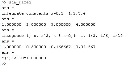
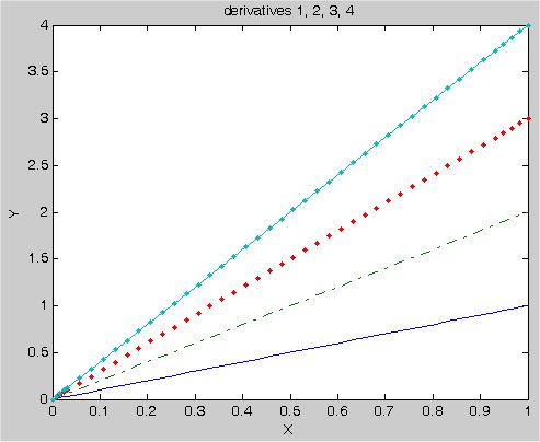
Systems of ordinary differential equations
The system of differential equations is N equations in N dependent
variables, Y, with one independent variable X.
Y_i = Y'_i(X, Y_1, Y_2, ... , Y_N) for i=1,N
The user provides the code for the functions Y'_i and places
the results in the F array. X goes from initial value, set by user,
to XLIM final value set by user. The user initializes the Y_i.
sim_difeq.f90 Fortran version
sim_difeq_f90.out
sim_difeq.java Java version
sim_difeq_java.out close to same results
sim_difeq.c C version
sim_difeq_c.out close to same results
sim_difeq.m MatLab version (main)
ode_test1.m funct computes derivatives
ode_test4.m funct computes derivatives
more ordinary differential equations for Matlab solution
ode_1.m sample 1
ode_2.m sample 2
move0.m for sample 2
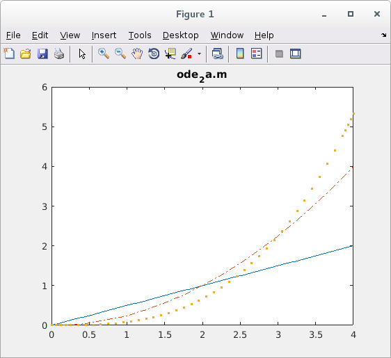
ode_2a.m sample 2a
 ode_3.m sample 3
ode_4.m sample 4
ode_5.m sample 5
ode_6a.m sample 6
ode_3.m sample 3
ode_4.m sample 4
ode_5.m sample 5
ode_6a.m sample 6
 ode_6a.m sample 6
 A brief look at definitions (we will cover more later)
See differential equations definitions .
A brief look at definitions (we will cover more later)
See differential equations definitions .
<- previous index next ->
-
CMSC 455 home page
-
Syllabus - class dates and subjects, homework dates, reading assignments
-
Homework assignments - the details
-
Projects -
-
Partial Lecture Notes, one per WEB page
-
Partial Lecture Notes, one big page for printing
-
Downloadable samples, source and executables
-
Some brief notes on Matlab
-
Some brief notes on Python
-
Some brief notes on Fortran 95
-
Some brief notes on Ada 95
-
An Ada math library (gnatmath95)
-
Finite difference approximations for derivatives
-
MATLAB examples, some ODE, some PDE
-
parallel threads examples
-
Reference pages on Taylor series, identities,
coordinate systems, differential operators
-
selected news related to numerical computation