<- previous index next ->
Spice is one of a number of electrical circuit simulation programs.
Our UMBC computers have a version called ngspice installed.
This is an example of a transient analysis, computed by integration
in small time steps. Similar to our rocket simulation.
Spice circuit input
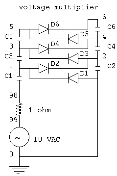
capdio.cir voltage multiplier ngspice -b capdio.cir > capdio.out
VS 99 0 AC 10 SIN(0VOFF 10VPEAK 1KHZ)
R1 99 98 1
C1 98 1 1UF
C2 0 2 1UF
C3 1 3 1UF
C4 2 4 1UF
C5 3 5 1UF
C6 4 6 1UF
D1 0 1
D2 1 2
D3 2 3
D4 3 4
D5 4 5
D6 5 6
.TRAN 100US 50MS
.print tran V(1) V(2) V(3) V(4) V(5) V(6)
.plot tran V(1) V(2) V(3) V(4) V(5) V(6)
.end
The schematic diagram with node numbers is:
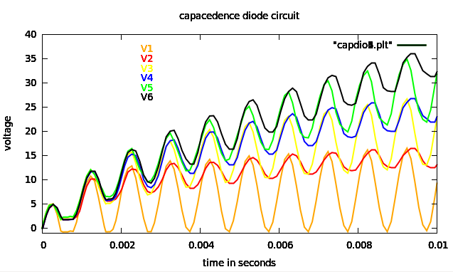
 The simulation with time step of 100 microseconds
for 0.01 seconds shows the voltage buildup at
the six nodes 1, 2, 3, 4, 5, 6 in the circuit.
The simulation with time step of 100 microseconds
for 0.01 seconds shows the voltage buildup at
the six nodes 1, 2, 3, 4, 5, 6 in the circuit.
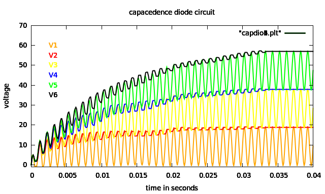
 Running the simulation to 0.04 seconds shows
stable voltage at node 6.
Running the simulation to 0.04 seconds shows
stable voltage at node 6.
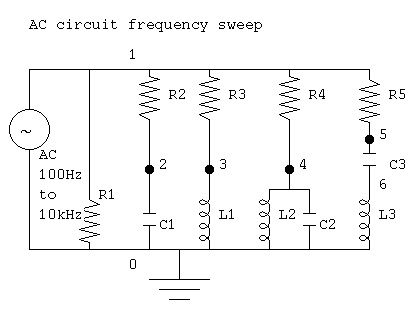
 Another type of Spice simulation is to simulate
a circuit at a series of frequencies. Type AC.
After setup of a matrix, solve simultaneous
equations to compute results.
Spice circuit input
ac.cir ac tuned circuit ngspice -b ac.cir > ac.out
I 0 1 ac 1000.0
R1 0 1 0.001
R2 1 2 1000.0
R3 1 3 1000.0
R4 1 4 1000.0
R5 1 5 1000.0
C1 2 0 0.0000001591549431
L1 3 0 0.1591549431
C2 4 0 0.0000001591549431
L2 4 0 0.1591549431
C3 5 6 0.0000001591549431
L3 6 0 0.1591549431
*F1 10.0 100000.0 10.0
.ac DEC 20 100 10k $ 100Hz to 10kHz, 20 points per decade
.print AC V(1) V(2) V(3) V(4) V(5)
.plot AC V(2) V(3) V(4) V(5)
.end
Another type of Spice simulation is to simulate
a circuit at a series of frequencies. Type AC.
After setup of a matrix, solve simultaneous
equations to compute results.
Spice circuit input
ac.cir ac tuned circuit ngspice -b ac.cir > ac.out
I 0 1 ac 1000.0
R1 0 1 0.001
R2 1 2 1000.0
R3 1 3 1000.0
R4 1 4 1000.0
R5 1 5 1000.0
C1 2 0 0.0000001591549431
L1 3 0 0.1591549431
C2 4 0 0.0000001591549431
L2 4 0 0.1591549431
C3 5 6 0.0000001591549431
L3 6 0 0.1591549431
*F1 10.0 100000.0 10.0
.ac DEC 20 100 10k $ 100Hz to 10kHz, 20 points per decade
.print AC V(1) V(2) V(3) V(4) V(5)
.plot AC V(2) V(3) V(4) V(5)
.end
 Some of the output from ac.out showing magnitude of
signal at nodes 2, 3, 4, 5 with frequency from
100Hz to 10kHz, note where frequency matches
the parallel tuned circuit at node 4,
and the series tuned circuit at node 5,
at 1kHz.
Note node 2, the capacitor C1 has low impedance at high frequency.
Note node 3. the inductor L1 has high impedance at high frequency.
Circuit: ac.cir ac tuned circuit ngspice -b ac.cir > ac.out
selected output from ac.out
Legend: + = v(2) * = v(3) X = multiple nodes
= = v(4) $ = v(5)
--------------------------------------------------------------------------
frequency v(2) 0.00e+00 2.00e-01 4.00e-01 6.00e-01 8.00e-01 1.00e+00
----------------------|---------|---------|---------|---------|---------|
1.000e+02 9.901e-01 X . . . . X.
1.122e+02 9.876e-01 X . . . . X.
1.259e+02 9.844e-01 X . . . . X.
1.413e+02 9.804e-01 *= . . . . $+.
1.585e+02 9.755e-01 .X . . . . X .
1.778e+02 9.693e-01 .X . . . . X .
1.995e+02 9.617e-01 .*= . . . . $+ .
2.239e+02 9.523e-01 . X . . . . X .
2.512e+02 9.406e-01 . *= . . . . $+ .
2.818e+02 9.264e-01 . *= . . . . $+ .
3.162e+02 9.091e-01 . *= . . . . $+ .
3.548e+02 8.882e-01 . * = . . . . $ + .
3.981e+02 8.632e-01 . * =. . . $ + .
4.467e+02 8.337e-01 . * .= . . $ .+ .
5.012e+02 7.992e-01 . * = . . $ +. .
5.623e+02 7.597e-01 . . * = $. + . .
6.310e+02 7.153e-01 . . * . $ = . + . .
7.079e+02 6.661e-01 . . X . . X . .
7.943e+02 6.131e-01 . $ . *. + .= .
8.913e+02 5.573e-01 . $ . . * + . . = .
1.000e+03 5.000e-01 $ . . X . . =.
1.122e+03 4.427e-01 . $ . . + * . . = .
1.259e+03 3.869e-01 . $ . +. * .= .
1.413e+03 3.339e-01 . . X . . X . .
1.585e+03 2.847e-01 . . + . $ = . * . .
1.778e+03 2.403e-01 . . + = $. * . .
1.995e+03 2.008e-01 . + = . . $ *. .
2.239e+03 1.663e-01 . + .= . . $ .* .
2.512e+03 1.368e-01 . + =. . . $ * .
2.818e+03 1.118e-01 . + = . . . . $ * .
3.162e+03 9.091e-02 . += . . . . $* .
3.548e+03 7.359e-02 . += . . . . $* .
3.981e+03 5.935e-02 . += . . . . $* .
4.467e+03 4.773e-02 . X . . . . X .
5.012e+03 3.829e-02 .+= . . . . $* .
5.623e+03 3.065e-02 .X . . . . X .
6.310e+03 2.450e-02 .X . . . . X .
7.079e+03 1.956e-02 += . . . . $*.
7.943e+03 1.560e-02 X . . . . X.
8.913e+03 1.243e-02 X . . . . X.
1.000e+04 9.901e-03 X . . . . X.
----------------------|---------|---------|---------|---------|---------|
frequency v(2) 0.00e+00 2.00e-01 4.00e-01 6.00e-01 8.00e-01 1.00e+00
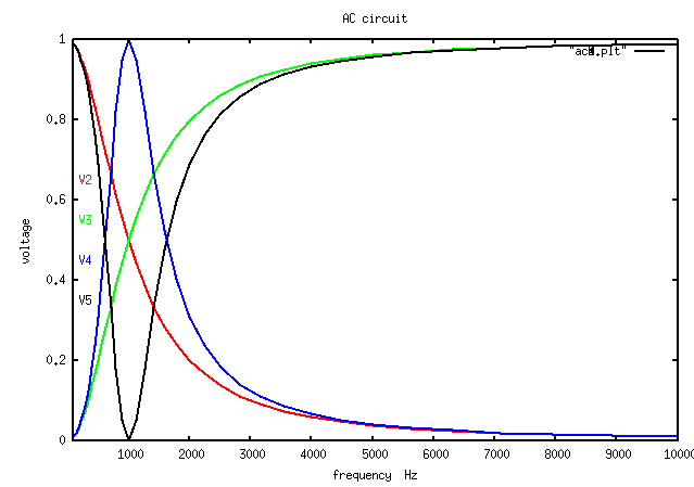
Then, nodes 2, 3, 4, 5 plotted on linear frequency scale
Some of the output from ac.out showing magnitude of
signal at nodes 2, 3, 4, 5 with frequency from
100Hz to 10kHz, note where frequency matches
the parallel tuned circuit at node 4,
and the series tuned circuit at node 5,
at 1kHz.
Note node 2, the capacitor C1 has low impedance at high frequency.
Note node 3. the inductor L1 has high impedance at high frequency.
Circuit: ac.cir ac tuned circuit ngspice -b ac.cir > ac.out
selected output from ac.out
Legend: + = v(2) * = v(3) X = multiple nodes
= = v(4) $ = v(5)
--------------------------------------------------------------------------
frequency v(2) 0.00e+00 2.00e-01 4.00e-01 6.00e-01 8.00e-01 1.00e+00
----------------------|---------|---------|---------|---------|---------|
1.000e+02 9.901e-01 X . . . . X.
1.122e+02 9.876e-01 X . . . . X.
1.259e+02 9.844e-01 X . . . . X.
1.413e+02 9.804e-01 *= . . . . $+.
1.585e+02 9.755e-01 .X . . . . X .
1.778e+02 9.693e-01 .X . . . . X .
1.995e+02 9.617e-01 .*= . . . . $+ .
2.239e+02 9.523e-01 . X . . . . X .
2.512e+02 9.406e-01 . *= . . . . $+ .
2.818e+02 9.264e-01 . *= . . . . $+ .
3.162e+02 9.091e-01 . *= . . . . $+ .
3.548e+02 8.882e-01 . * = . . . . $ + .
3.981e+02 8.632e-01 . * =. . . $ + .
4.467e+02 8.337e-01 . * .= . . $ .+ .
5.012e+02 7.992e-01 . * = . . $ +. .
5.623e+02 7.597e-01 . . * = $. + . .
6.310e+02 7.153e-01 . . * . $ = . + . .
7.079e+02 6.661e-01 . . X . . X . .
7.943e+02 6.131e-01 . $ . *. + .= .
8.913e+02 5.573e-01 . $ . . * + . . = .
1.000e+03 5.000e-01 $ . . X . . =.
1.122e+03 4.427e-01 . $ . . + * . . = .
1.259e+03 3.869e-01 . $ . +. * .= .
1.413e+03 3.339e-01 . . X . . X . .
1.585e+03 2.847e-01 . . + . $ = . * . .
1.778e+03 2.403e-01 . . + = $. * . .
1.995e+03 2.008e-01 . + = . . $ *. .
2.239e+03 1.663e-01 . + .= . . $ .* .
2.512e+03 1.368e-01 . + =. . . $ * .
2.818e+03 1.118e-01 . + = . . . . $ * .
3.162e+03 9.091e-02 . += . . . . $* .
3.548e+03 7.359e-02 . += . . . . $* .
3.981e+03 5.935e-02 . += . . . . $* .
4.467e+03 4.773e-02 . X . . . . X .
5.012e+03 3.829e-02 .+= . . . . $* .
5.623e+03 3.065e-02 .X . . . . X .
6.310e+03 2.450e-02 .X . . . . X .
7.079e+03 1.956e-02 += . . . . $*.
7.943e+03 1.560e-02 X . . . . X.
8.913e+03 1.243e-02 X . . . . X.
1.000e+04 9.901e-03 X . . . . X.
----------------------|---------|---------|---------|---------|---------|
frequency v(2) 0.00e+00 2.00e-01 4.00e-01 6.00e-01 8.00e-01 1.00e+00
Then, nodes 2, 3, 4, 5 plotted on linear frequency scale
<- previous index next ->