<- previous index next ->
The goal of this lecture is to have the student understand how
to numerically compute the solution of a differential equation.
The numerical solution will be computed by a computer program.
Almost any computer language can be used to compute the numerical
solution of differental equations. Various languages will be
used as examples. Much of the notation will be more computer
programming oriented than mathematical.
This lecture starts with very basic concepts and defines the notation
that will be used.
Expect terms to be defined close to the terms first usage.
We start with ordinary differential equations and then cover
partial differential equations.
An ordinary differential equation has exactly one independent
variable, typically x .
A partial differential equation has more than one independent
variable, typically x,y x,y,z x,y,z,t etc.
understanding derivatives
From a numerical point of view, the derivative of
a function is the slope at a specific value for the
independent variable.
The second derivative is just the derivative of
the first derivative of a function.
Note*** first a polynomial, then the sine
we know from Calculus:
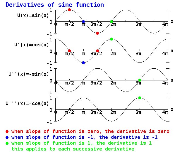
U(x) = sin(x)
U'(x) d/dx sin(x) = cos(x) the first derivative od sine x is cosine x
U''(x) d/dx cos(x) = -sin(x) the second derivative of sine x is -sine x
U'''(x) d/dx -sin(x) = -cos(x) the third derivative of sine x is -cosine x
Look at the plot of sin(x) and its derivatives.
Note the slope of each curve at each point, is the derivative
plotted below it. A few are highlighted by red, blue and
green dots.
notation for ordinary differential equations
f(x) A function of x, typically any function of one independent variable.
x^3 + 7 x^2 + 5 x + 4 is a polynomial function of x,
x cubed plus 7 times x squared plus 5 times x plus 4 .
sin(x) a function of x that computes the sine of x .
All trignometric functions will use x in radians.
y=f(x) an equation, some times written y = f(x);
y'(x)=3 x^2 + 14 x + 5; y(0)=4;
A differential equation with an initial condition.
The analytic solution is f(x) the polynomial above.
Given y=f(x) , y'(x) is the notation for taking
the first derivative of f(x),
also written as d/dx f(x) or d f(x)/dx .
Typically we are given a starting and ending value
for which the numerical solution is needed.
The result may be a table of x,y values and
often a graphical plot of the solution.
y''''(x)-y(x)=0; y(0)=0; y'(0)=1; y''(0)=0; y'''(0)=-1;
A fourth order differential equation with initial conditions.
We will see later why four initial conditions are
needed in order to compute the numerical solution.
We know the analytic solution is f(x)=sin(x);
yet we will see that we must be careful of errors
in computing the numerical solution.
a(x)*y'' + b(x)*y' + c(x) = 0 is a second order ordinary
differential equation. The three functions a(x),
b(x), and c(x) must be known and programmable.
In general functions will appear more than
constants in differential equations.
notation for partial differential equations
f(x,y,z) a function of three independent variables.
2*x*y^2*z + 4*x^2*z^2 + 3*y
a polynomial in three variables
2 times x times y squared times z plus
4 times x squared times z squared plus 3 time y
U(x,y,z) will be the numerical solution of a partial differential
equation giving values of f(x,y,z) in a specified three
dimensional region.
Ux(x,y,z) or just Ux if the independent variables are obvious,
is the first derivative with respect to x of f(x,y,z) .
Uxx is the second derivative with respect to x of f(x,y,z)
Uxy is the first derivative with respect to x of f(x,y,z)=Ux
then the first derivative with respect to y of Ux.
Uxyyz is the first derivative with respect to x, then the
second derivative with respect to y, then the first
derivative with respect to z.
Uxxx + a(x,y,z)*Uyyz + b(x,y,z)*Uz = c(x,y,z);
Is a partial differential equation.
In order to numerically solve this equation we need
the three functions a(x,y,z), b(x,y,z) and c(x,y,z)
to be specified and we must be able to code them
in the programming language we wish to use to
compute the numerical solution.
Typically this type of partial differential equation
has a closed three dimensional volume, called the
boundary, where the solution must be computed.
Enough values of the function f(x,y,z) must be
given, typically on the boundary, to have a
unique solution defined. These values are known
as Dirchilet boundary values. Derivative values
may also be provided on the boundary, these are
known as Neumann boundary values.
required conditions
In order to compute a unique numerical solution we need:
1) The function f that is the solution must be continuous
and continuously differentiable in and on the boundary.
(Solving for discontinuous results, such as shock waves
is beyond the scope of this tutorial.)
2) There must be enough boundary values to make the
solution unique. At least one Dirichilet value must
be given and possibly some number of Neumann values.
3) The boundary must be given. For this tutorial we
cover only one closed boundary with no internal "holes".
4) The coordinate system is assumed Cartesian unless
otherwise specified, Polar, Cylindrical, Spherical,
Elipsoidal, or other.
numerically solving our first ordinary differential equation
<- previous index next ->