<- previous index next ->
The message here:
Thoroughly test any software you write or are about to use.
Use tools to generate test when possible.
Generate a test case for a second order PDE with two independent variables.
Make the PDE general by having it be elliptic in some regions,
hyperbolic in some regions and passing through parabolic.
Note: This is for the set of solutions that are continuous and
continuously differentiable. There are many special solutions and
corresponding special solvers that should be used for special cases.
This lecture is about a general case and a general solver.
The solution will be u(x,y).
The notation for derivatives will be
uxx(x,y) second derivative of u(x,y) with respect to x
uxy(x,y) derivative of u(x,y) with respect to x and with respect to y
uyy(x,y) second derivative of u(x,y) with respect to
ux(x,y) derivative of u(x,y) with respect to x
uy(x,y) derivative of u(x,y) with respect to y
We will create functions a1(x,y), b1(x,y), c1(x,y), d1(x,y), e1(x,y) and
f1(x,y).
The PDE we intend to solve, compactly, is:
a1 uxx + b1 uxy + c1 uyy + d1 ux + e1 uy + f1 u = c
The PDE written for computer processing is:
a1(x,y)*uxx(x,y) + b1(x,y)*uxy(x,y) + c1(x,y)*uyy(x,y) +
d1(x,y)*ux(x,y) + e1(x,y)*uy(x,y) + f1(x,y)*u(x,y) = c(x,y)
Yes, we could use algebra to reorganize the PDE, yet we will not.
We choose the functions a1, b1 and c1 such that b1^2 -a1 * c1 is
elliptic, hyperbolic and parabolic in various regions.
a1(x,y) = exp(x/2)*exp(y)/2
b1(x,y) = 0.7/(x*x*y*y + 0.5)
c1(x,y) = (4 - exp(x) - exp(y/2))*2
then we plot b1^2 - a1 * c1 over the x-y plane.
abc.m MatLab to plot a1, b1, c1 and b1^2-a1*c1
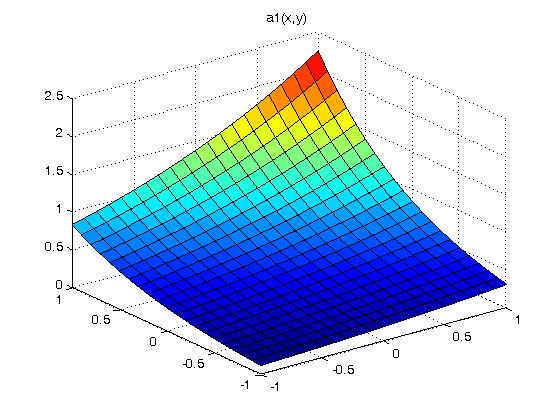
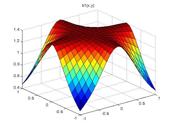
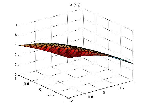
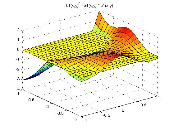 Below the yellow plane is elliptic, above the yellow plane is
hyperbolic and on the yellow plane is parabolic. This has little
to do with the numerical solution of our PDE. For some classic
PDE's only in one region, there are specialized solutions.
Equations of mixed type:
If a PDE has coefficients which are not constant, as shown above,
it is possible that it will not belong to any of the three categories.
A simple but important example is the Euler-Tricomi equation
uxx = xuyy
which is called elliptic-hyperbolic because it is elliptic in the region
x < 0, hyperbolic in the region x > 0, and degenerate parabolic
on the line x = 0.
The other functions for this test case were chosen as:
d1(x,y) = x^2 y
e1(x,y) = x y^2
f1(x,y) = 3x + 2y
Now we have to pick our solution function u(x,y).
Since we will be taking second derivatives, we need at least a
third order solution in order to be interesting.
Out of the air, I chose:
u(x,y) = x^3 + 2y^3 + 3x^2 y + 4xy^2 + 5xy + 6x + 7y + 8
We do not want the solution symmetric in x and y.
We want a smattering of terms for testing.
I use 1, 2, 3, 4, ... to be sure each term tested.
Now we have to compute the forcing function c(x,y)
Doing the computation by hand is too error prone.
I use Maple.
Maple computation of c(x,y) Look at this!
Maple work sheet
Maple output
c(x,y) = 0.5*exp(x/2.0)*exp(y)*(6.0*x+6.0*y) +
0.7*(6.0*x + 8.0*y + 5.0)/(x*x*y*y+0.5) +
(8.0 - 2.0*exp(x) - 2.0*exp(y/2.0))*(12.0*y + 8.0*x) +
(x*x+y)*(3.0*x*x + 6.0*x*y + 4.0*y*y + 5.0*y + 6.0) +
x*y*y*(6.0*y*y + 3.0*x*x + 8.0*x*y + 5.0*x +7.0) +
(3.0*x + 2.0*y)*(x^3 + 2y^3 + 3x^2 y + 4xy^2 + 5xy + 6x + 7y + 8)
We have to code the function c(x,y) for our solver.
We have to code the function u(x,y) for our solver to compute
boundary values and we will use the function to check our solver.
The solution will be u(x,y) and the solver must be able to evaluate
this function on the boundary. The region will be
xmin <= x <= xmax
ymin <= y <= ymax
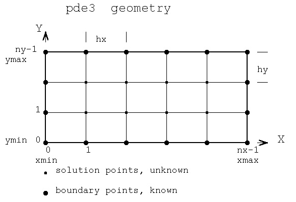
We will solve for nx points in the x dimension, ny points in y dimension with
hx=(xmax-xmin)/(nx-1) step size in x
hy=(ymax-ymin)/(ny-1) step size in y
We will compute the approximate solution at u(i,j) for the point
u(xmin+i*hx,ymin+j*hy). With subscripts running i=0..nx-1 and j=0..ny-1.
Known boundary values are at i=0, i=nx-1, j=0, and j=ny-1.
These subscripts are for "C" and Java, add one for Ada, Fortran and
MatLab subscripts.
The actual numeric values can be set at the last minute, yet we will
use xmin = ymin = -1.0 xmax = ymax = 1.0 nx = 7 ny = 7
Now, we have to generate the matrix that represents the system of
linear simultaneous equations for the unknown values of u(x,y)
at xmin+i*hx for i=1..nx-2 ymin+j*hy for j=1..ny-2
I am using solution points 1, 2, ... , nx-2 by
1, 2, ... , ny-2 stored in a matrix starting at ut[0][0] for coding in "C".
The solution points will be the same as used in pde3:
Below the yellow plane is elliptic, above the yellow plane is
hyperbolic and on the yellow plane is parabolic. This has little
to do with the numerical solution of our PDE. For some classic
PDE's only in one region, there are specialized solutions.
Equations of mixed type:
If a PDE has coefficients which are not constant, as shown above,
it is possible that it will not belong to any of the three categories.
A simple but important example is the Euler-Tricomi equation
uxx = xuyy
which is called elliptic-hyperbolic because it is elliptic in the region
x < 0, hyperbolic in the region x > 0, and degenerate parabolic
on the line x = 0.
The other functions for this test case were chosen as:
d1(x,y) = x^2 y
e1(x,y) = x y^2
f1(x,y) = 3x + 2y
Now we have to pick our solution function u(x,y).
Since we will be taking second derivatives, we need at least a
third order solution in order to be interesting.
Out of the air, I chose:
u(x,y) = x^3 + 2y^3 + 3x^2 y + 4xy^2 + 5xy + 6x + 7y + 8
We do not want the solution symmetric in x and y.
We want a smattering of terms for testing.
I use 1, 2, 3, 4, ... to be sure each term tested.
Now we have to compute the forcing function c(x,y)
Doing the computation by hand is too error prone.
I use Maple.
Maple computation of c(x,y) Look at this!
Maple work sheet
Maple output
c(x,y) = 0.5*exp(x/2.0)*exp(y)*(6.0*x+6.0*y) +
0.7*(6.0*x + 8.0*y + 5.0)/(x*x*y*y+0.5) +
(8.0 - 2.0*exp(x) - 2.0*exp(y/2.0))*(12.0*y + 8.0*x) +
(x*x+y)*(3.0*x*x + 6.0*x*y + 4.0*y*y + 5.0*y + 6.0) +
x*y*y*(6.0*y*y + 3.0*x*x + 8.0*x*y + 5.0*x +7.0) +
(3.0*x + 2.0*y)*(x^3 + 2y^3 + 3x^2 y + 4xy^2 + 5xy + 6x + 7y + 8)
We have to code the function c(x,y) for our solver.
We have to code the function u(x,y) for our solver to compute
boundary values and we will use the function to check our solver.
The solution will be u(x,y) and the solver must be able to evaluate
this function on the boundary. The region will be
xmin <= x <= xmax
ymin <= y <= ymax
We will solve for nx points in the x dimension, ny points in y dimension with
hx=(xmax-xmin)/(nx-1) step size in x
hy=(ymax-ymin)/(ny-1) step size in y
We will compute the approximate solution at u(i,j) for the point
u(xmin+i*hx,ymin+j*hy). With subscripts running i=0..nx-1 and j=0..ny-1.
Known boundary values are at i=0, i=nx-1, j=0, and j=ny-1.
These subscripts are for "C" and Java, add one for Ada, Fortran and
MatLab subscripts.
The actual numeric values can be set at the last minute, yet we will
use xmin = ymin = -1.0 xmax = ymax = 1.0 nx = 7 ny = 7
Now, we have to generate the matrix that represents the system of
linear simultaneous equations for the unknown values of u(x,y)
at xmin+i*hx for i=1..nx-2 ymin+j*hy for j=1..ny-2
I am using solution points 1, 2, ... , nx-2 by
1, 2, ... , ny-2 stored in a matrix starting at ut[0][0] for coding in "C".
The solution points will be the same as used in pde3:
 The PDE will be made discrete by using unknown values in difference
equations as given in nderiv.out or
computed by deriv.c, deriv.adb, deriv.java, deriv.py, deriv.scala, etc.
For this test case, I choose to use five point derivatives for
both first and second order. Note that the uxy term has the
first derivative with respect to x at five y values then
the first derivative of these values with respect to y.
Taking a term at a time from the PDE and writing the discrete version:
a1(x,y)*uxx(x,y) + b1(x,y)*uxy(x,y) + c1(x,y)*uyy(x,y) +
d1(x,y)*ux(x,y) + e1(x,y)*uy(x,y) + f1(x,y)*u(x,y) = c(x,y)
At (x,y) the discrete approximation of a1(x,y)*uxx(x,y) =
a1(x,y) * (1/(12*hx*hx)) *
(-1*u(x-2hx,y) +16*u(x-hx,y) -30*u(x,y) +16*u(x+hx,y) -1*u(x+2hx,y))
yet, we want to solve for u(i,j) in a matrix,
thus using x=xmin+i*hx and y=ymin+j*hy rewrite the above approximation as
a1(xmin+i*hx,ymin+j*hy) * (1/(12*hx*hx)) *
(-1*u(i-2,j) +16*u(i-1,j) -30*u(i,j) +16*u(i+1,j) -1*u(i+2,j))
At (x,y) c1(x,y)*uyy(x,y) = the discrete approximation
c1(x,y) * (1/(12*hy*hy)) *
(-1*u(x,y-2hy) +16*u(x,y-hy) -30*u(x,y) +16*u(x,y+hy) -1*u(x,y+2hy))
again, we want to solve for u(i,j) in a matrix,
thus using x=xmin+i*hx and y=ymin+j*hy rewrite the above approximation as
c1(xmin+i*hx,ymin+j*hy) * (1/(12*hy*hy)) *
(-1*u(i,j-2) +16*u(i,j-1) -30*u(i,j) +16*u(i,j+1) -1*u(i,j+2))
What happened to b1(x,y)*uxy(x,y) ?
Well that one is more difficult, thus we now use the combination of
the first derivative with respect to x, then the first derivative
with respect to y, 25 terms.
Writing all the terms using i and j
b1(xmin+i*hx,ymin+j*hy) * (1/(144*hx*hy)) *
( 1*u(i-2,j-2) -8*u(i-1,j-2) +0*u(i,j-2) +8*u(i+1,j-2) -1*u(i+2,j-2)
-8*u(i-2,j-1) +64*u(i-1,j-1) +0*u(i,j-1) -64*u(i+1,j-1) +8*u(i+2,j-1)
+0*u(i-2,j ) +0*u(i-1,j ) +0*u(i,j ) +0*u(i+1,j ) +0*u(i+2,j )
+8*u(i-2,j+1) -64*u(i-1,j+1) +0*u(i,j+1) +64*u(i+1,j+1) -8*u(i+2,j+1)
-1*u(i-2,j+2) +8*u(i-1,j+2) +0*u(i,j+2) -8*u(i+1,j+2) +1*u(i+2,j+2))
Just writing the remaining terms using i and j
using the discrete coefficients.
d1(xmin+i*hx,ymin+j*hy) * (1/(12*hx) *
(1*u(i-2,j) -8*u(i-1,j) +0*u(i,j) +8*u(i+1,j) -1*u(i+2,j))
e1(xmin+i*hx,ymin+j*hy) * (1/(12*hy) *
(1*u(i,j-2) -8*u(i,j-1) +0*u(i,j) +8*u(i,j+1) -1*u(i,j+2))
The u(x,y) term is just
f1(xmin+i*hx,ymin+j*hy)*u(i,j)
The right hand side of every approximation above is just
c(xmin+i*hx,ymin+j*hy)
If any of the u(i+a,j+b) are boundary elements, we plug in the
numeric value of the boundary element, multiply by the
coefficient, and subtract the product from the right hand side.
Now we have many equations for u(i,j) using values for i and j,
and we must compute the coefficients for the set of equations
for i=2..nx-3 j=2..ny-3 the central case.
Remember, u(i=0,j), u(i=nx-1,j), u(i,j=0) and u(i,j=ny-1) are
known boundary values.
What about u(1,j), u(nx-2,j) for j=1..ny-2 and
u(i,1), u(i,ny-2) for i=2..nx-3 (do not use u(1,1) twice !!!)
(do not use u(nx-2,ny-2) twice)
Fortunately, the coefficients for the discrete derivatives can be
computed by deriv.c, deriv.adb, etc.
At (1,j) the discrete approximation of
a1(xmin+1*hx,ymin*j*hy)*uxx(xmin+1*hx,ymin+j*hy) =
a1(xmin+1*hx,ymin+j*hy) * (1/(12*hx*hx)) *
(-3*u(i-1,j) -10*u(i,j) +18*u(i+1,j) -6*u(i+2,j) +1*u(i+3,j))
We could not use i-2 because it is outside our region, thus
note "deriv" is called with 'point' set to 1.
At (nx-2,j) the discrete approximation of
a1(xmin+(nx-2)*hx,ymin*j*hy)*uxx(xmin+(nx-2)*hx,ymin+j*hy) =
a1(xmin+(nx-2)*hx,ymin+j*hy) * (1/(12*hx*hx)) *
(-1*u(i-3,j) +6*u(i-2,j) -18*u(i-1,j) +10*u(i,j) +3*u(i+1,j))
We could not use i+2 or (nx-2)+2 because it is outside our region, thus
note "deriv" is called with 'point' set to 3.
There is nothing special about uxx(i,1) or uxx(nx-2,1) use the general case.
At (i,1) the discrete approximation of c1(x,y)*uyy(x,y) =
c1(xmin+i*hx,ymin+1*hy) * (1/(12*hy*hy)) *
(-3*u(i,j-1) -10*u(i,j) +18*u(i,j+1) -6*u(i,j+2) +1*u(i,j+3))
We could not use j-2 because it is outside our region, thus
note "deriv" is called with 'point' set to 1.
At (i,nx-2) the discrete approximation of c1(x,y)*uyy(x,y) =
c1(xmin+i*hx,ymin+(nx-2)*hy) * (1/(12*hy*hy)) *
(-1*u(i,j-3) +6*u(i,j-2) -18*u(i,j-1) +10*u(i,j) +3*u(i,j+1))
We could not use j+2 or (ny-2)+2 because it is outside our region, thus
note "deriv" is called with 'point' set to 3.
There is nothing special about uyy(1,j) or uxx(nx-2,j) use the general case.
Oh, and yes, ux(x,y) uy(x,y) uxy(x,y) also have to be shifted for the
"just inside the boundary case." Think of how much easier it is using five
points rather than sever points. With seven points the two rows and
columns inside the boundary are special cases.
Now we have enough equations to exactly compute the approximate solution.
We build a system of linear equations of the form:
| ut00 ut01 ut02 ut03 | | u(1,1) | | k0 |
| ut10 ut11 ut12 ut13 | * | u(1,2) | = | k1 |
| ut20 ut21 ut22 ut23 | | u(2,1) | | k2 |
| ut30 ut31 ut32 ut33 | | u(2,2) | | k3 |
We know the values at the boundary u(0,0), u(0,1), u(0,2), u(0,3)
u(1,0), u(1,3)
u(2,0), u(2,3)
u(3,0), u(3,1), u(3,2), u(3,3)
For this specific system of equations, nx=4, ny=4 and there are four
internal, non boundary, values to be found. The number of equations
will always be (nx-2)*(ny-2).
The value found for u(1,1) from solving the system of linear equations
is the desired solution at u(xmin+1*hx,ymin+1*hy). u(2,2) is the value of
u(xmin+2*hx,ymin+2*hy). Additional values, not on hx or hy steps,
of u(x,y) may be found by two dimensional interpolation.
The matrix "ut", used in the source code pde_abc_eq.c
is cleared to zero. Then each equation is used and the
coefficient of u(i,j) is added the appropriate ut entry.
There will be (nx-2)*(ny-2) equations that must be used.
The i and j for these equations are for i=1..nx-2 for j=1..ny-2.
The PDE approximation above must be used for these i,j pairs.
Note that u(i,j), u(i-2,j) etc are variables and it is the
coefficients of these variables that get added into the "ut" matrix.
The first equation will add to entries in the first row of the matrix.
The second equation will add to entries in the second row of the matrix.
The boundary values are not stored in the ut matrix and using algebra,
a boundary value coefficient is multiplied by the boundary value and
subtracted from the constant term. This can cause many special cases
in the solver.
In general many entries in a row will not be changed from zero.
The final matrix will be in the class of a band matrix.
Now the gruesome work of evaluating the u(i,j) coefficients.
We cheat here. Now assume nx>4 and ny>5 and thus
i=2, j=3 is a general center case. From above, we have
a1(x,y)*uxx(x,y) + b1(x,y)*uxy(x,y) + c1(x,y)*uyy(x,y) +
d1(x,y)*ux(x,y) + e1(x,y)*uy(x,y) + f1(x,y)*u(x,y) = c(x,y)
converted to a discrete approximation for the central elements is
a1(xmin+i*hx,ymin+j*hy) * (1/(12*hx*hx)) *
(-1*u(i-2,j) +16*u(i-1,j) -30*u(i,j) +16*u(i+1,j) -1*u(i+2,j)) +
b1(xmin+i*hx,y+j*hy) * (1/(144*hx*hy)) *
( 1*u(i-2,j-2) -8*u(i-1,j-2) +0*u(i,j-2) +8*u(i+1,j-2) -1*u(i+2,j-2)
-8*u(i-2,j-1) +64*u(i-1,j-1) +0*u(i,j-1) -64*u(i+1,j-1) +8*u(i+2,j-1)
+0*u(i-2,j ) +0*u(i-1,j ) +0*u(i,j ) +0*u(i+1,j ) +0*u(i+2,j )
+8*u(i-2,j+1) -64*u(i-1,j+1) +0*u(i,j+1) +64*u(i+1,j+1) -8*u(i+2,j+1)
-1*u(i-2,j+2) +8*u(i-1,j+2) +0*u(i,j+2) -8*u(i+1,j+2) +1*u(i+2,j+2)) +
c1(xmin+i*hx,ymin+j*hy) * (1/(12*hy*hy)) *
(-1*u(i,j-2) +16*u(i,j-1) -30*u(i,j) +16*u(i,j+1) -1*u(i,j+2)) +
d1(xmin+i*hx,ymin+j*hy) * (1/(12*hx) *
(1*u(i-2,j) -8*u(i-1,j) +0*u(i,j) +8*u(i+1,j) -1*u(i+2,j)) +
e1(xmin+i*hx,ymin+j*hy) * (1/(12*hy) *
(1*u(i,j-2) -8*u(i,j-1) +0*u(i,j) +8*u(i,j+1) -1*u(i,j+2)) +
f1(xmin+i*hx,ymin+j*hy)*u(i,j) =
c(xmin+i*hx,ymin+j*hy)
Collecting terms for u(i,j) we compute the coefficient ct
a1(xmin+i*hx,ymin+j*hy) * (1/(12*hx*hx)) *(-30) +
b1(xmin+i*hx,ymin+j*hy) * (1/(144*hx*hy)) *(0) +
c1(xmin+i*hx,ymin+j*hy) * (1/(12*hy*hy)) *(-30) +
d1(xmin+i*hx,ymin+j*hy) * (1/(12*hx) *(0) +
e1(xmin+i*hx,ymin+j*hy) * (1/(12*hy) *(0)
and the right hand side is c(xmin+i*hx,ymin+j*hy)
A bit of bizarre subscripting, assuming we are at i=2, j=3 this
is equation number ii=(i-1)+(nx-2)*(j-1), right?
Check i=1,j=1 is equation 0 if i or j equal zero, we have a boundary
i=2,j=1 is equation 1
...
i=nx-2,j=1 is equation nx-3
i=1,j=2 is equation nx-2
i=2,j=2 is equation nx-1
...
i=2,j=3 is equation (2-1)+(nx-2)*(3-1) the row in the ut matrix.
cs, the subscript for the right hand side is cs=(nx-2)*(ny-2) stored in ut.
Thus we add ct to ut(ii,ii). The second subscript is where u(i,j) is.
Well, to tell the truth, we add each component of the sum in a loop,
directly into ut(ii,ii). If we had ct we would just store it in ut(ii,ii).
ut(ii,cs) is set to c(xmin+i*hx,ymin+j*hy) - f1(xmin+i*hx,ymin+j*hy)
We must, of course, compute all the coefficients, e.g. u(i-1,j), ctm1
a1(xmin+i*hx,ymin+j*hy) * (1/(12*hx*hx)) *(16) +
b1(xmin+i*hx,ymin+j*hy) * (1/(144*hx*hy)) *(0) +
c1(xmin+i*hx,ymin+j*hy) * (1/(12*hy*hy)) *(0) + does not exists
d1(xmin+i*hx,ymin+j*hy) * (1/(12*hx) *(-8) +
e1(xmin+i*hx,ymin+j*hy) * (1/(12*hy) *(0) does not exists
ij=(((i-1)-1)+(nx-2)*(j-1) where u(i-1,j) is in the solution vector.
ut(ii,ij) = ctm1
We must, of course, compute all the coefficients, e.g. u(i-2,j), ctmm1
a1(xmin+i*hx,ymin+j*hy) * (1/(12*hx*hy)) *(-1) +
b1(xmin+i*hx,ymin+j*hy) * (1/(144*hx*hy)) *(0) +
c1(xmin+i*hx,ymin+j*hy) * (1/(12*hy*hy)) *(0) + does not exists
d1(xmin+i*hx,ymin+j*hy) * (1/(12*hx) *(1) +
e1(xmin+i*hx,ymin+j*hy) * (1/(12*hy) *(0) does not exists
ij=(((i-2)-1)+(nx-2)*(j-1) where u(i-2,j) is in the solution vector.
ut(ii,ij) = ctmm1 Wrong if i is 2! u(0,j) is a boundary value, thus
ut(ii,cs) = ut(ii,cs) - ctmm1 * u(0,j)
And, one more coefficients, e.g. u(i,j+1), ctp1
a1(xmin+i*hx,ymin+j*hy) * (1/(12*hx*hx)) *(0) + does not exists
b1(xmin+i*hx,ymin+j*hy) * (1/(144*hx*hy)) *(0) +
c1(xmin+i*hx,ymin+j*hy) * (1/(12*hy*hy)) *(16) +
d1(xmin+i*hx,ymin+j*hy) * (1/(12*hx) *(0 ) + does not exists
e1(xmin+i*hx,ymin+j*hy) * (1/(12*hy) *(8)
"C" and Java subscripting
ij=((i-1)+(nx-2)*((j+1)-1) when u(i,j+1) is in the solution vector.
ut(ii,ij) = ctp1
Ada, Fortran and MatLab subscripting
ij=(i-1)+(nx-2)*((j+1)-2) when u(i,j+1) is in the solution vector.
ut(ii,ij) = ctp1
where uc(ii) is the right hand side.
Yes, the code is nested four levels deep in iterations.
Now do u(1,j), u(nx-2,j) for j=1..ny-2 and
u(i,1), u(i,ny-2) for i=2..nx-3 (do not use u(1,1) twice !!!)
(do not use u(nx-2,ny-2) twice)
Once the "ut" matrix is initialized, solve the simultaneous equations
and print the answers. Now, wasn't that easy.
A crude layout for nx=9, ny=9 is shown below with subscripts
The i,j notation is for a known boundary value,
the number is the ii subscript of the unknown value inside the I====I
I ut I
I====I.
j
0 1 2 3 4 5 6 7 8 ny=9
+-----------------------------------------------------+
0 | 0,0 | 0,1 | 0,2 | 0,3 | 0,4 | 0,5 | 0,6 | 0,7 | 0,8 |
| I=========================================I |
1 | 1,0 I 0 | 7 | 14 | 21 | 28 | 35 | 42 I 1,8 |
| I-----------------------------------------I |
2 | 2,0 I 1 | 8 | 15 | 22 | 29 | 36 | 43 I 2,8 |
| I-----------------------------------------I |
3 | 3,0 I 2 | 9 | 16 | 23 | 30 | 37 | 44 I 3,8 |
| I-----------------------------------------I |
i 4 | 4,0 I 3 | 10 | 17 | 24 | 31 | 38 | 45 I 4,8 |
| I-----------------------------------------I |
5 | 5,0 I 4 | 11 | 18 | 25 | 32 | 39 | 46 I 5,8 |
| I-----------------------------------------I |
6 | 6,0 I 5 | 12 | 19 | 26 | 33 | 40 | 47 I 6,8 |
| I-----------------------------------------I |
7 | 7,0 I 6 | 13 | 20 | 27 | 34 | 41 | 48 I 7,8 |
| I=========================================I |
8 | 8,0 | 8,1 | 8,2 | 8,3 | 8,4 | 8,5 | 8,6 | 8,7 | 8,8 |
+-----------------------------------------------------+
nx=9
ut(ii) where ii = (i-1)+(nx-2)*(j-1)
These are "C" and Java subscripts.
j
1 2 3 4 5 6 7 8 9 ny=9
+-----------------------------------------------------+
1 | 1,1 | 1,2 | 1,3 | 1,4 | 1,5 | 1,6 | 1,7 | 1,8 | 1,9 |
| I=========================================I |
2 | 2,1 I 1 | 8 | 15 | 22 | 29 | 36 | 43 I 2,9 |
| I-----------------------------------------I |
3 | 3,1 I 2 | 9 | 16 | 23 | 30 | 37 | 44 I 3,9 |
| I-----------------------------------------I |
4 | 4,1 I 3 | 10 | 17 | 24 | 31 | 38 | 45 I 4,9 |
| I-----------------------------------------I |
i 5 | 5,1 I 4 | 11 | 18 | 25 | 32 | 39 | 46 I 5,9 |
| I-----------------------------------------I |
6 | 6,1 I 5 | 12 | 19 | 26 | 33 | 40 | 47 I 6,9 |
| I-----------------------------------------I |
7 | 7,1 I 6 | 13 | 20 | 27 | 34 | 41 | 48 I 7,9 |
| I-----------------------------------------I |
8 | 8,1 I 7 | 14 | 21 | 28 | 35 | 42 | 49 I 8,9 |
| I=========================================I |
9 | 9,1 | 9,2 | 9,3 | 9,4 | 9,5 | 9,6 | 9,7 | 9,8 | 9,9 |
+-----------------------------------------------------+
nx=9
ut(ii) where ii = (i-1)+(nx-2)*(j-2)
These are Ada, Fortran and Matlab subscripts.
A differential equation that has regions hyperbolic, elliptic and parabolic
defined in the various languages "abc" file.
The basic functions coded in "C" for this test case are:
abc.txt instructions for user
abc.h sample test case described above
abc.c implementation of test case
deriv.h discretization header file
deriv.c discretization
pde_abc_eq.c solver program
pde_abc_eq_c.out sample output
abc.c implementation of test case
The basic functions coded in Fortran 90 for this test case are:
abc.f90 implementation of test case
deriv.f90 discretization
simeq.f90 solve simultaneous equations
pde_abc_eq.f90 solver program
pde_abc_eq_f90.out sample output
The basic functions coded in Java for this test case are:
abc.java sample test case described above
nderiv.java discretization
simeq.java solve simultaneous equations
pde_abc_eq.java solver program
pde_abc_eq_java.out sample output
The basic functions coded in Ada 95 for this test case are:
abc.ads sample test case described above
abc.adb implementation of test case
deriv.adb discretization
rderiv.adb discretization
simeq.adb solve simultaneous equations
pde_abc_eq.adb solver program
pde_abc_eq_ada.out sample output
Sparse matrix storage is needed for the system of linear equations
when nx or ny is significantly greater than the discretization
order, nd.
The same PDE's as above, using the definition in "abc" are
easily modified to use sparse matrix storage and a direct
sparse matrix solution to the linear equations.
The basic functions coded in "C" for this test case are:
abc.txt instructions for user
sparse.h sparse matrix header file
sparse.c sparse matrix for PDE's
deriv.h discretization header file
deriv.c discretization
abc.h sample test case described above
abc.c implementation of test case
sparse_abc.c sparse solver program
sparse_abc_c.out sample output
The basic functions coded in Java for this test case are:
abc.java sample test case described above
sparse.java sparse matrix for PDE's
nderiv.java discretization
sparse_abc.java solver program
sparse_abc_java.out sample output
The basic functions coded in Ada 95 for this test case are:
abc.ads sample test case described above
abc.adb implementation of test case
sparse.ads sparse matrix specification
sparse.adb sparse matrix for PDE's
deriv.adb discretization
sparse_abc.adb solver program
sparse_abc_ada.out sample output
Some challenging fourth order partial differential equations
including biharmonic equations
are covered in lecture 28d
Solving nonlinear PDE is covered in Lecture 31b.
The specific case for the nonlinear Navier Stokes Equations is
covered in Lecture 28b
For nonlinear PDE to be solved by solving a system of equations,
the simultaneous equations are non linear.
To solve a system of nonlinear equations reasonably efficiently,
use a Jacobian matrix and an iterative solution.
An example that can handle up to third order nonlinear systems of
equations is shown by using a Newton iteration based on the inverse
of the Jacobian:
x_next = x_prev - J^-1 * ( A * x_prev - Y)
simeq_newton3.java basic solver
test_simeq_newton3.java test program
test_simeq_newton3_java.out test_output
on three test cases (minor heuristic used to build J)
The PDE will be made discrete by using unknown values in difference
equations as given in nderiv.out or
computed by deriv.c, deriv.adb, deriv.java, deriv.py, deriv.scala, etc.
For this test case, I choose to use five point derivatives for
both first and second order. Note that the uxy term has the
first derivative with respect to x at five y values then
the first derivative of these values with respect to y.
Taking a term at a time from the PDE and writing the discrete version:
a1(x,y)*uxx(x,y) + b1(x,y)*uxy(x,y) + c1(x,y)*uyy(x,y) +
d1(x,y)*ux(x,y) + e1(x,y)*uy(x,y) + f1(x,y)*u(x,y) = c(x,y)
At (x,y) the discrete approximation of a1(x,y)*uxx(x,y) =
a1(x,y) * (1/(12*hx*hx)) *
(-1*u(x-2hx,y) +16*u(x-hx,y) -30*u(x,y) +16*u(x+hx,y) -1*u(x+2hx,y))
yet, we want to solve for u(i,j) in a matrix,
thus using x=xmin+i*hx and y=ymin+j*hy rewrite the above approximation as
a1(xmin+i*hx,ymin+j*hy) * (1/(12*hx*hx)) *
(-1*u(i-2,j) +16*u(i-1,j) -30*u(i,j) +16*u(i+1,j) -1*u(i+2,j))
At (x,y) c1(x,y)*uyy(x,y) = the discrete approximation
c1(x,y) * (1/(12*hy*hy)) *
(-1*u(x,y-2hy) +16*u(x,y-hy) -30*u(x,y) +16*u(x,y+hy) -1*u(x,y+2hy))
again, we want to solve for u(i,j) in a matrix,
thus using x=xmin+i*hx and y=ymin+j*hy rewrite the above approximation as
c1(xmin+i*hx,ymin+j*hy) * (1/(12*hy*hy)) *
(-1*u(i,j-2) +16*u(i,j-1) -30*u(i,j) +16*u(i,j+1) -1*u(i,j+2))
What happened to b1(x,y)*uxy(x,y) ?
Well that one is more difficult, thus we now use the combination of
the first derivative with respect to x, then the first derivative
with respect to y, 25 terms.
Writing all the terms using i and j
b1(xmin+i*hx,ymin+j*hy) * (1/(144*hx*hy)) *
( 1*u(i-2,j-2) -8*u(i-1,j-2) +0*u(i,j-2) +8*u(i+1,j-2) -1*u(i+2,j-2)
-8*u(i-2,j-1) +64*u(i-1,j-1) +0*u(i,j-1) -64*u(i+1,j-1) +8*u(i+2,j-1)
+0*u(i-2,j ) +0*u(i-1,j ) +0*u(i,j ) +0*u(i+1,j ) +0*u(i+2,j )
+8*u(i-2,j+1) -64*u(i-1,j+1) +0*u(i,j+1) +64*u(i+1,j+1) -8*u(i+2,j+1)
-1*u(i-2,j+2) +8*u(i-1,j+2) +0*u(i,j+2) -8*u(i+1,j+2) +1*u(i+2,j+2))
Just writing the remaining terms using i and j
using the discrete coefficients.
d1(xmin+i*hx,ymin+j*hy) * (1/(12*hx) *
(1*u(i-2,j) -8*u(i-1,j) +0*u(i,j) +8*u(i+1,j) -1*u(i+2,j))
e1(xmin+i*hx,ymin+j*hy) * (1/(12*hy) *
(1*u(i,j-2) -8*u(i,j-1) +0*u(i,j) +8*u(i,j+1) -1*u(i,j+2))
The u(x,y) term is just
f1(xmin+i*hx,ymin+j*hy)*u(i,j)
The right hand side of every approximation above is just
c(xmin+i*hx,ymin+j*hy)
If any of the u(i+a,j+b) are boundary elements, we plug in the
numeric value of the boundary element, multiply by the
coefficient, and subtract the product from the right hand side.
Now we have many equations for u(i,j) using values for i and j,
and we must compute the coefficients for the set of equations
for i=2..nx-3 j=2..ny-3 the central case.
Remember, u(i=0,j), u(i=nx-1,j), u(i,j=0) and u(i,j=ny-1) are
known boundary values.
What about u(1,j), u(nx-2,j) for j=1..ny-2 and
u(i,1), u(i,ny-2) for i=2..nx-3 (do not use u(1,1) twice !!!)
(do not use u(nx-2,ny-2) twice)
Fortunately, the coefficients for the discrete derivatives can be
computed by deriv.c, deriv.adb, etc.
At (1,j) the discrete approximation of
a1(xmin+1*hx,ymin*j*hy)*uxx(xmin+1*hx,ymin+j*hy) =
a1(xmin+1*hx,ymin+j*hy) * (1/(12*hx*hx)) *
(-3*u(i-1,j) -10*u(i,j) +18*u(i+1,j) -6*u(i+2,j) +1*u(i+3,j))
We could not use i-2 because it is outside our region, thus
note "deriv" is called with 'point' set to 1.
At (nx-2,j) the discrete approximation of
a1(xmin+(nx-2)*hx,ymin*j*hy)*uxx(xmin+(nx-2)*hx,ymin+j*hy) =
a1(xmin+(nx-2)*hx,ymin+j*hy) * (1/(12*hx*hx)) *
(-1*u(i-3,j) +6*u(i-2,j) -18*u(i-1,j) +10*u(i,j) +3*u(i+1,j))
We could not use i+2 or (nx-2)+2 because it is outside our region, thus
note "deriv" is called with 'point' set to 3.
There is nothing special about uxx(i,1) or uxx(nx-2,1) use the general case.
At (i,1) the discrete approximation of c1(x,y)*uyy(x,y) =
c1(xmin+i*hx,ymin+1*hy) * (1/(12*hy*hy)) *
(-3*u(i,j-1) -10*u(i,j) +18*u(i,j+1) -6*u(i,j+2) +1*u(i,j+3))
We could not use j-2 because it is outside our region, thus
note "deriv" is called with 'point' set to 1.
At (i,nx-2) the discrete approximation of c1(x,y)*uyy(x,y) =
c1(xmin+i*hx,ymin+(nx-2)*hy) * (1/(12*hy*hy)) *
(-1*u(i,j-3) +6*u(i,j-2) -18*u(i,j-1) +10*u(i,j) +3*u(i,j+1))
We could not use j+2 or (ny-2)+2 because it is outside our region, thus
note "deriv" is called with 'point' set to 3.
There is nothing special about uyy(1,j) or uxx(nx-2,j) use the general case.
Oh, and yes, ux(x,y) uy(x,y) uxy(x,y) also have to be shifted for the
"just inside the boundary case." Think of how much easier it is using five
points rather than sever points. With seven points the two rows and
columns inside the boundary are special cases.
Now we have enough equations to exactly compute the approximate solution.
We build a system of linear equations of the form:
| ut00 ut01 ut02 ut03 | | u(1,1) | | k0 |
| ut10 ut11 ut12 ut13 | * | u(1,2) | = | k1 |
| ut20 ut21 ut22 ut23 | | u(2,1) | | k2 |
| ut30 ut31 ut32 ut33 | | u(2,2) | | k3 |
We know the values at the boundary u(0,0), u(0,1), u(0,2), u(0,3)
u(1,0), u(1,3)
u(2,0), u(2,3)
u(3,0), u(3,1), u(3,2), u(3,3)
For this specific system of equations, nx=4, ny=4 and there are four
internal, non boundary, values to be found. The number of equations
will always be (nx-2)*(ny-2).
The value found for u(1,1) from solving the system of linear equations
is the desired solution at u(xmin+1*hx,ymin+1*hy). u(2,2) is the value of
u(xmin+2*hx,ymin+2*hy). Additional values, not on hx or hy steps,
of u(x,y) may be found by two dimensional interpolation.
The matrix "ut", used in the source code pde_abc_eq.c
is cleared to zero. Then each equation is used and the
coefficient of u(i,j) is added the appropriate ut entry.
There will be (nx-2)*(ny-2) equations that must be used.
The i and j for these equations are for i=1..nx-2 for j=1..ny-2.
The PDE approximation above must be used for these i,j pairs.
Note that u(i,j), u(i-2,j) etc are variables and it is the
coefficients of these variables that get added into the "ut" matrix.
The first equation will add to entries in the first row of the matrix.
The second equation will add to entries in the second row of the matrix.
The boundary values are not stored in the ut matrix and using algebra,
a boundary value coefficient is multiplied by the boundary value and
subtracted from the constant term. This can cause many special cases
in the solver.
In general many entries in a row will not be changed from zero.
The final matrix will be in the class of a band matrix.
Now the gruesome work of evaluating the u(i,j) coefficients.
We cheat here. Now assume nx>4 and ny>5 and thus
i=2, j=3 is a general center case. From above, we have
a1(x,y)*uxx(x,y) + b1(x,y)*uxy(x,y) + c1(x,y)*uyy(x,y) +
d1(x,y)*ux(x,y) + e1(x,y)*uy(x,y) + f1(x,y)*u(x,y) = c(x,y)
converted to a discrete approximation for the central elements is
a1(xmin+i*hx,ymin+j*hy) * (1/(12*hx*hx)) *
(-1*u(i-2,j) +16*u(i-1,j) -30*u(i,j) +16*u(i+1,j) -1*u(i+2,j)) +
b1(xmin+i*hx,y+j*hy) * (1/(144*hx*hy)) *
( 1*u(i-2,j-2) -8*u(i-1,j-2) +0*u(i,j-2) +8*u(i+1,j-2) -1*u(i+2,j-2)
-8*u(i-2,j-1) +64*u(i-1,j-1) +0*u(i,j-1) -64*u(i+1,j-1) +8*u(i+2,j-1)
+0*u(i-2,j ) +0*u(i-1,j ) +0*u(i,j ) +0*u(i+1,j ) +0*u(i+2,j )
+8*u(i-2,j+1) -64*u(i-1,j+1) +0*u(i,j+1) +64*u(i+1,j+1) -8*u(i+2,j+1)
-1*u(i-2,j+2) +8*u(i-1,j+2) +0*u(i,j+2) -8*u(i+1,j+2) +1*u(i+2,j+2)) +
c1(xmin+i*hx,ymin+j*hy) * (1/(12*hy*hy)) *
(-1*u(i,j-2) +16*u(i,j-1) -30*u(i,j) +16*u(i,j+1) -1*u(i,j+2)) +
d1(xmin+i*hx,ymin+j*hy) * (1/(12*hx) *
(1*u(i-2,j) -8*u(i-1,j) +0*u(i,j) +8*u(i+1,j) -1*u(i+2,j)) +
e1(xmin+i*hx,ymin+j*hy) * (1/(12*hy) *
(1*u(i,j-2) -8*u(i,j-1) +0*u(i,j) +8*u(i,j+1) -1*u(i,j+2)) +
f1(xmin+i*hx,ymin+j*hy)*u(i,j) =
c(xmin+i*hx,ymin+j*hy)
Collecting terms for u(i,j) we compute the coefficient ct
a1(xmin+i*hx,ymin+j*hy) * (1/(12*hx*hx)) *(-30) +
b1(xmin+i*hx,ymin+j*hy) * (1/(144*hx*hy)) *(0) +
c1(xmin+i*hx,ymin+j*hy) * (1/(12*hy*hy)) *(-30) +
d1(xmin+i*hx,ymin+j*hy) * (1/(12*hx) *(0) +
e1(xmin+i*hx,ymin+j*hy) * (1/(12*hy) *(0)
and the right hand side is c(xmin+i*hx,ymin+j*hy)
A bit of bizarre subscripting, assuming we are at i=2, j=3 this
is equation number ii=(i-1)+(nx-2)*(j-1), right?
Check i=1,j=1 is equation 0 if i or j equal zero, we have a boundary
i=2,j=1 is equation 1
...
i=nx-2,j=1 is equation nx-3
i=1,j=2 is equation nx-2
i=2,j=2 is equation nx-1
...
i=2,j=3 is equation (2-1)+(nx-2)*(3-1) the row in the ut matrix.
cs, the subscript for the right hand side is cs=(nx-2)*(ny-2) stored in ut.
Thus we add ct to ut(ii,ii). The second subscript is where u(i,j) is.
Well, to tell the truth, we add each component of the sum in a loop,
directly into ut(ii,ii). If we had ct we would just store it in ut(ii,ii).
ut(ii,cs) is set to c(xmin+i*hx,ymin+j*hy) - f1(xmin+i*hx,ymin+j*hy)
We must, of course, compute all the coefficients, e.g. u(i-1,j), ctm1
a1(xmin+i*hx,ymin+j*hy) * (1/(12*hx*hx)) *(16) +
b1(xmin+i*hx,ymin+j*hy) * (1/(144*hx*hy)) *(0) +
c1(xmin+i*hx,ymin+j*hy) * (1/(12*hy*hy)) *(0) + does not exists
d1(xmin+i*hx,ymin+j*hy) * (1/(12*hx) *(-8) +
e1(xmin+i*hx,ymin+j*hy) * (1/(12*hy) *(0) does not exists
ij=(((i-1)-1)+(nx-2)*(j-1) where u(i-1,j) is in the solution vector.
ut(ii,ij) = ctm1
We must, of course, compute all the coefficients, e.g. u(i-2,j), ctmm1
a1(xmin+i*hx,ymin+j*hy) * (1/(12*hx*hy)) *(-1) +
b1(xmin+i*hx,ymin+j*hy) * (1/(144*hx*hy)) *(0) +
c1(xmin+i*hx,ymin+j*hy) * (1/(12*hy*hy)) *(0) + does not exists
d1(xmin+i*hx,ymin+j*hy) * (1/(12*hx) *(1) +
e1(xmin+i*hx,ymin+j*hy) * (1/(12*hy) *(0) does not exists
ij=(((i-2)-1)+(nx-2)*(j-1) where u(i-2,j) is in the solution vector.
ut(ii,ij) = ctmm1 Wrong if i is 2! u(0,j) is a boundary value, thus
ut(ii,cs) = ut(ii,cs) - ctmm1 * u(0,j)
And, one more coefficients, e.g. u(i,j+1), ctp1
a1(xmin+i*hx,ymin+j*hy) * (1/(12*hx*hx)) *(0) + does not exists
b1(xmin+i*hx,ymin+j*hy) * (1/(144*hx*hy)) *(0) +
c1(xmin+i*hx,ymin+j*hy) * (1/(12*hy*hy)) *(16) +
d1(xmin+i*hx,ymin+j*hy) * (1/(12*hx) *(0 ) + does not exists
e1(xmin+i*hx,ymin+j*hy) * (1/(12*hy) *(8)
"C" and Java subscripting
ij=((i-1)+(nx-2)*((j+1)-1) when u(i,j+1) is in the solution vector.
ut(ii,ij) = ctp1
Ada, Fortran and MatLab subscripting
ij=(i-1)+(nx-2)*((j+1)-2) when u(i,j+1) is in the solution vector.
ut(ii,ij) = ctp1
where uc(ii) is the right hand side.
Yes, the code is nested four levels deep in iterations.
Now do u(1,j), u(nx-2,j) for j=1..ny-2 and
u(i,1), u(i,ny-2) for i=2..nx-3 (do not use u(1,1) twice !!!)
(do not use u(nx-2,ny-2) twice)
Once the "ut" matrix is initialized, solve the simultaneous equations
and print the answers. Now, wasn't that easy.
A crude layout for nx=9, ny=9 is shown below with subscripts
The i,j notation is for a known boundary value,
the number is the ii subscript of the unknown value inside the I====I
I ut I
I====I.
j
0 1 2 3 4 5 6 7 8 ny=9
+-----------------------------------------------------+
0 | 0,0 | 0,1 | 0,2 | 0,3 | 0,4 | 0,5 | 0,6 | 0,7 | 0,8 |
| I=========================================I |
1 | 1,0 I 0 | 7 | 14 | 21 | 28 | 35 | 42 I 1,8 |
| I-----------------------------------------I |
2 | 2,0 I 1 | 8 | 15 | 22 | 29 | 36 | 43 I 2,8 |
| I-----------------------------------------I |
3 | 3,0 I 2 | 9 | 16 | 23 | 30 | 37 | 44 I 3,8 |
| I-----------------------------------------I |
i 4 | 4,0 I 3 | 10 | 17 | 24 | 31 | 38 | 45 I 4,8 |
| I-----------------------------------------I |
5 | 5,0 I 4 | 11 | 18 | 25 | 32 | 39 | 46 I 5,8 |
| I-----------------------------------------I |
6 | 6,0 I 5 | 12 | 19 | 26 | 33 | 40 | 47 I 6,8 |
| I-----------------------------------------I |
7 | 7,0 I 6 | 13 | 20 | 27 | 34 | 41 | 48 I 7,8 |
| I=========================================I |
8 | 8,0 | 8,1 | 8,2 | 8,3 | 8,4 | 8,5 | 8,6 | 8,7 | 8,8 |
+-----------------------------------------------------+
nx=9
ut(ii) where ii = (i-1)+(nx-2)*(j-1)
These are "C" and Java subscripts.
j
1 2 3 4 5 6 7 8 9 ny=9
+-----------------------------------------------------+
1 | 1,1 | 1,2 | 1,3 | 1,4 | 1,5 | 1,6 | 1,7 | 1,8 | 1,9 |
| I=========================================I |
2 | 2,1 I 1 | 8 | 15 | 22 | 29 | 36 | 43 I 2,9 |
| I-----------------------------------------I |
3 | 3,1 I 2 | 9 | 16 | 23 | 30 | 37 | 44 I 3,9 |
| I-----------------------------------------I |
4 | 4,1 I 3 | 10 | 17 | 24 | 31 | 38 | 45 I 4,9 |
| I-----------------------------------------I |
i 5 | 5,1 I 4 | 11 | 18 | 25 | 32 | 39 | 46 I 5,9 |
| I-----------------------------------------I |
6 | 6,1 I 5 | 12 | 19 | 26 | 33 | 40 | 47 I 6,9 |
| I-----------------------------------------I |
7 | 7,1 I 6 | 13 | 20 | 27 | 34 | 41 | 48 I 7,9 |
| I-----------------------------------------I |
8 | 8,1 I 7 | 14 | 21 | 28 | 35 | 42 | 49 I 8,9 |
| I=========================================I |
9 | 9,1 | 9,2 | 9,3 | 9,4 | 9,5 | 9,6 | 9,7 | 9,8 | 9,9 |
+-----------------------------------------------------+
nx=9
ut(ii) where ii = (i-1)+(nx-2)*(j-2)
These are Ada, Fortran and Matlab subscripts.
A differential equation that has regions hyperbolic, elliptic and parabolic
defined in the various languages "abc" file.
The basic functions coded in "C" for this test case are:
abc.txt instructions for user
abc.h sample test case described above
abc.c implementation of test case
deriv.h discretization header file
deriv.c discretization
pde_abc_eq.c solver program
pde_abc_eq_c.out sample output
abc.c implementation of test case
The basic functions coded in Fortran 90 for this test case are:
abc.f90 implementation of test case
deriv.f90 discretization
simeq.f90 solve simultaneous equations
pde_abc_eq.f90 solver program
pde_abc_eq_f90.out sample output
The basic functions coded in Java for this test case are:
abc.java sample test case described above
nderiv.java discretization
simeq.java solve simultaneous equations
pde_abc_eq.java solver program
pde_abc_eq_java.out sample output
The basic functions coded in Ada 95 for this test case are:
abc.ads sample test case described above
abc.adb implementation of test case
deriv.adb discretization
rderiv.adb discretization
simeq.adb solve simultaneous equations
pde_abc_eq.adb solver program
pde_abc_eq_ada.out sample output
Sparse matrix storage is needed for the system of linear equations
when nx or ny is significantly greater than the discretization
order, nd.
The same PDE's as above, using the definition in "abc" are
easily modified to use sparse matrix storage and a direct
sparse matrix solution to the linear equations.
The basic functions coded in "C" for this test case are:
abc.txt instructions for user
sparse.h sparse matrix header file
sparse.c sparse matrix for PDE's
deriv.h discretization header file
deriv.c discretization
abc.h sample test case described above
abc.c implementation of test case
sparse_abc.c sparse solver program
sparse_abc_c.out sample output
The basic functions coded in Java for this test case are:
abc.java sample test case described above
sparse.java sparse matrix for PDE's
nderiv.java discretization
sparse_abc.java solver program
sparse_abc_java.out sample output
The basic functions coded in Ada 95 for this test case are:
abc.ads sample test case described above
abc.adb implementation of test case
sparse.ads sparse matrix specification
sparse.adb sparse matrix for PDE's
deriv.adb discretization
sparse_abc.adb solver program
sparse_abc_ada.out sample output
Some challenging fourth order partial differential equations
including biharmonic equations
are covered in lecture 28d
Solving nonlinear PDE is covered in Lecture 31b.
The specific case for the nonlinear Navier Stokes Equations is
covered in Lecture 28b
For nonlinear PDE to be solved by solving a system of equations,
the simultaneous equations are non linear.
To solve a system of nonlinear equations reasonably efficiently,
use a Jacobian matrix and an iterative solution.
An example that can handle up to third order nonlinear systems of
equations is shown by using a Newton iteration based on the inverse
of the Jacobian:
x_next = x_prev - J^-1 * ( A * x_prev - Y)
simeq_newton3.java basic solver
test_simeq_newton3.java test program
test_simeq_newton3_java.out test_output
on three test cases (minor heuristic used to build J)
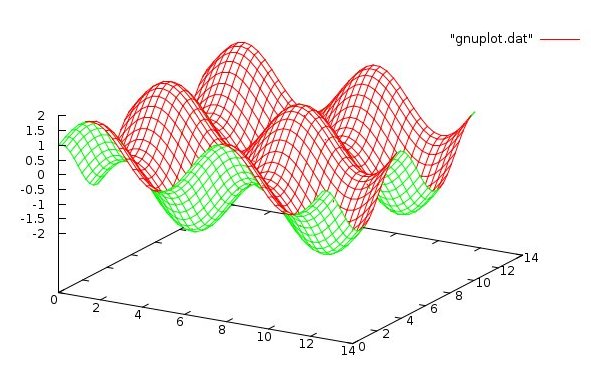
Plotting Solutions
Plotting solutions can be easy with Linux and gnuplot.
To demonstrate, I have a program that generates a 2D solution
that needs a 3D plot. make_gnuplotdata.c
The data file, for this case, is gnuplot.dat
The input file to gnuplot is my2.plot
The shell script to make the plot is test2_gnuplot.sh
The plot is run by typing sh test2_gnuplot.sh
or from inside a program with test2_gnuplot.c
or from command line gnuplot -persist my2.plot
The result is the plot
A special case is tests for Laplace Equation
ΔU = 0 or ∇2U = 0 or Uxx(x,y) + Uyy(x,y) = 0 or
∂2U/∂x2 + ∂2U/∂y2 = 0
Many known solutions and thus Dirichlet boundary conditions
for test cases are known:
k>0 is any constant
U(x,y)=k
U(x,y)=k*x
U(x,y)=k*y
U(x,y)=k*x*y
U(x,y)=k*x^2 - k*y^2
U(x,y)=sin(k*x)*sinh(k*y)
U(x,y)=sin(k*x)*cosh(k*y)
U(x,y)=cos(k*x)*sinh(k*y)
U(x,y)=cos(k*x)*cosh(k*y)
U(x,y)=sin(k*x)*exp( k*y)
U(x,y)=sin(k*x)*exp(-k*y)
U(x,y)=cos(k*x)*exp( k*y)
U(x,y)=cos(k*x)*exp(-k*y)
r=sqrt(x^2+y^2)
th=atan2(y,x) -Pi..Pi principal value is
U(x,y)=r^k * sin(k*th) discontinuous along negative X axis
using atan2 in 0..2Pi wrong!
causes discontinuous derivative along positive X axis
<- previous index next ->
-
CMSC 455 home page
-
Syllabus - class dates and subjects, homework dates, reading assignments
-
Homework assignments - the details
-
Projects -
-
Partial Lecture Notes, one per WEB page
-
Partial Lecture Notes, one big page for printing
-
Downloadable samples, source and executables
-
Some brief notes on Matlab
-
Some brief notes on Python
-
Some brief notes on Fortran 95
-
Some brief notes on Ada 95
-
An Ada math library (gnatmath95)
-
Finite difference approximations for derivatives
-
MATLAB examples, some ODE, some PDE
-
parallel threads examples
-
Reference pages on Taylor series, identities,
coordinate systems, differential operators
-
selected news related to numerical computation