<- previous index next ->
Simultaneous equations are multiple equations involving the same
variables. In general, to get a unique solution we need the
same number of equations as the number of unknown variables,
and the equations mutually linearly independent.
A sample set of three equations in three unknowns is:
eq1: 2*x + 3*y + 2*z = 13
eq2: 3*x + 2*y + 3*z = 17
eq3: 4*x - 2*y + 2*z = 12
One systematic solution method is called the Gauss-Jordan reduction.
We will reduce the three equations such that eq1: has only x,
eq2: has only y and eq3: has only z making the constant yield
the solution. Operations are always based on the latest version
of each equation. The numeric solution will perform the same
operations on a matrix.
Reduce the coefficient of x in the first equation to 1, dividing by 2
eq1: 1*x + 1.5*y + 1*z = 6.5
Eliminate the variable x from eq2: by subtracting eq2 coefficient of
x times eq1:
eq2: becomes eq2: - 3* eq1:
eq2: (3-3)*x + (2-4.5)*y + (3-3)*z = (17-19.5) then simplifying
eq2: 0*x - 2.5*y + 0*z = -2.5
Eliminate the variable x from eq3: by subtracting eq3 coefficient of
x times eq1:
eq3: becomes eq3: - 4* eq1:
eq3: (4-4)*x (-2 -6)*y + (2-4)*z = (12-26) then becomes
eq3: 0*x - 8*y - 2*z = -14
The three equations are now
eq1: 1*x + 1.5*y + 1*z = 6.5
eq2: 0*x - 2.5*y + 0*z = - 2.5
eq3: 0*x - 8.0*y - 2*z = -14.0
Reduce the coefficient of y in eq2: to 1, dividing by -2.5
eq2: 0*x + 1*y + 0*z = 1
Eliminate the variable y from eq1: by subtracting eq1 coefficient of y times eq2:
eq1: becomes eq1: -1.5* eq2:
eq1: 1*x + 0*y + 1*z = (6.5-1.5) then becomes
eq1: 1*x + 0*y + 1*z = 5
Eliminate the variable y from eq3: by subtracting eq3 coefficient of y times eq2:
eq3: becomes eq3: -8* eq2:
eq3: 0*x + 0*y - 2*z = (-14 +8) then becomes
eq3: 0*x + 0*y - 2*z = -6
The three equations are now
eq1: 1*x + 0*y + 1*z = 5
eq2: 0*x + 1*y + 0*z = 1
eq3: 0*x + 0*y - 2*z = -6
Reduce the coefficient of z in eq3: to 1, dividing by -2
eq3: 0*x + 0*y + 1*z = 3
Eliminate the variable z from eq1: by subtracting eq1 coefficient of z times eq2:
eq1: becomes eq1: -1* eq2:
eq1: 1*x + 0*y + 0*z = (5-3) then becomes
eq1: 1*x + 0*y + 0*z = 2
Eliminate the variable z from eq2: by subtracting eq2 coefficient of z times eq2:
eq2: becomes eq3: 0* eq2:
eq2: 0*x + 1*y + 0*z = 1
The three equations are now
eq1: 1*x + 0*y + 0*z = 2 or x = 2
eq2: 0*x + 1*y + 0*z = 1 or y = 1
eq3: 0*x + 0*y + 1*z = 3 or z = 3 the desired solution.
The numerical solution simply places the values in a matrix and uses the same
reductions shown above.
Given the equations: |A|*|X| = |Y| B = |AY|
eq1: 2*x + 3*y + 2*z = 13 | 2 3 2 | |x| |13|
eq2: 3*x + 2*y + 3*z = 17 | 3 2 3 |*|y|=|17|
eq3: 4*x - 2*y + 2*z = 12 | 4 -2 2 | |z| |12|
Create the matrix | 2 3 2 13 | having 3 rows and 4 columns
B = | 3 2 3 17 |
| 4 -2 2 12 |
The following code, using n=3 for these three equations, computes the
same desired solution as the manual method above.
for k=1:n
for j=k+1:n
B(k,j) = B(k,j)/B(k,k)
end
for i=1:n
if(i not k)
for j=1:n
B(i,j) = B(i,j) - B(i,k)*B(k,J)
Pivoting to avoid zero on diagonal and improve accuracy
Now we must consider the possible problem of B(k,k) being zero
for some value of k. It is rather obvious that the order of the
equations does not matter. The equations can be given in any
order and we get the same solution. Thus, simply interchange
any equation where we are about to divide by a zero B(k,k)
with some equation below that would not result in a zero B(k,k).
It turns out that we get better accuracy if we always pick
the equation that has the largest absolute value for B(k,k).
If the largest value turns out to be zero then there is no
unique solution for the set of equations.
We generally want numerical code to run efficiently and thus we
will not physically interchange the equations but rather keep
a row index array that tells us where the k th row is now.
The code for the final algorithm is given in the links below.
Note types of errors
test_simeq_small.c source code
test_simeq_small_c.out output
test_simeq_small.c results should be exactly X[0]=1.0, X[1]=-1.0
err is the error multiplying the solution, X, times matrix A*X=Y
a small change in data gives a big change in solution.
the big change is not indicated by the computed error.
decimal .835*X[0] + .667*X[1] = .168 Y[0]
decimal .333*X[0] + .266*X[1] = .067 Y[1]
flt-pt 0.835000*X[0] + 0.667000*X[1] = 0.168000
flt-pt 0.333000*X[0] + 0.266000*X[1] = 0.067000
initialization complete, solving
solution X[0]=1.0, err=0
solution X[1]=-1.0, err=0 -- expected
now perturb Y[1] from .067 to .066, .001 change, and run again
flt-pt 0.835000*X[0] + 0.667000*X[1] = 0.168000 Y[0]
flt-pt 0.333000*X[0] + 0.266000*X[1] = 0.066000 Y[1] -- only change
solution X[0]=-666.0, err=0
solution X[1]=834.0, err=2.84217e-14 -- X[1] WOW!
notice computed errors are still small,
yet, the values of X[0] and X[1] are very different.
Typical problem with people and computers:
Often called garbage in, garbage out!
test_inverse_small.c source code
test_inverse_small_c.out output
We will see later, when the norm of the coefficients of
simultaneous equations is inverted, and the norm of the inverse
is different by many orders of magnitude, the system will be
called ill-conditioned.
solving for function values on a grid
Solving for unknown function values on a given x,y grid:
test_eqn1 2*U(x,y) = C(x,y)
test_eqn2 2*U(x,y) + 3*V(x,y) = C(x,y)
3*U(x,y) + 3*V(x,y) = D(x,y)
test eqn3 2*U(x,y) + 3*V(x,y) + 4*W(x,y) = C(x,y)
4*U(x,y) + 2*V(x,y) + 3*W(x,y) = D(x,y)
3*U(x,y) + 4*V(x,y) + 2*W(x,y) = E(x,y)
test_eqn1.java source code
test_eqn1_java.out source code
test_eqn2.java source code
test_eqn2_java.out source code
test_eqn3.java source code
test_eqn3_java.out source code
test_eqn33.java source code
test_eqn33_java.out source code
test_eqn1.py3 source code
test_eqn1_py3.out source code
test_eqn2.py3 source code
test_eqn2_py3.out source code
test_eqn3.py3 source code
test_eqn3_py3.out source code
test_eqn33.py3 source code
test_eqn33_py3.out source code
Later lecture covers non linear equations.
Working code in many languages
The instructor understands that some students have a strong
prejudice in favor of, or against, some programming languages.
After about 50 years of programming in about 50 programming
languages, the instructor finds that the difference between
programming languages is mostly syntactic sugar. Yet, since
students may be able to read some programming languages
easier than others, these examples are presented in "C",
Fortran 95, Java and Ada 95. The intent was to do a quick
translation, keeping most of the source code the same,
for the different languages. Style was not a consideration.
Some rearranging of the order was used when convenient.
The numerical results are almost exactly the same.
The same code has been programmed in "C", Fortran 95, Java and Ada 95 etc.
as shown below with file types .c, .f90, .java and .adb .rb .py .scala:
Note the .h for C offers the user choices.
simeq.c "C" language source code
simeq.h "C" header file
time_simeq.c "C" language source code
time_simeq.out output
simeq.f90 Fortran 95 source code
time_simeq.f90 Fortran 95 source code
time_simeq_f90_cs.out output
simeq.java Java source code
time_simeq.java Java source code
time_simeq_java.out output
simeq.cpp C++ language source code
simeq.hpp C++ header file
test_simeq.cpp C++ language source code
test_simeq_cpp.out output
simeq.adb Ada 95 source code
real_arrays.ads Ada 95 source code
real_arrays.adb Ada 95 source code
Simeq.rb Ruby class Simeq
test_simeq.rb Ruby source code
test_simeq_rb.out Ruby output
simeq in matrix.pm Perl package
test_matrix.pl Perl source code test
test_matrix_pl.out Perl output
simeq.m MATLAB source code
simeq_m.out MATLAB output
With Python and downloading numpy using linalg
test_solve.py Python source code
test_solve_py.out Python output
With Python using numpy and array
test_simeq.py Python source code
test_simeq_py.out Python output
test_simeq.py3 Python source code
test_simeq_py3.out Python output
test_matmul.py3 Python source code
test_matmul_py3.out Python output
With Scala using Random, very small errors
Simeq.scala Scala source code
TestSimeq.scala Scala source code
TestSimeq_scala.out Scala output
Many methods have been devised for solving simultaneous equations.
A sample is LU decomposition and Crout method.
LU decomposition with pivoting:
lup_decomp.f90 source code
lup_decomp_f90.out output
simeq_lup.h source code
simeq_lup.c source code
time_simeq_lup.c source code
time_simeq_lup_cs.out output
simeq_lup.java source code
time_simeq_lup.java source code
time_simeq_lup_java.out output
Crout method without pivoting, uses back substitution:
crout.adb source code
crout_ada.out output
crout.f90 source code
time_crout.f90 source code
time_crout_f90.out output
crout.h source code
crout.c source code
time_crout.c source code
time_crout.c source code
time_crout_c.out output
crout1.h source code
crout1.c source code
time_crout1.c source code
time_crout1_c.out output
crout.java source code
test_crout.java accuracy test source
test_crout_java.out output
crout1.java source code
time_crout.java accuracy test source
time_crout_java.out output
Back substitution:
The difference from plain Gauss-Jordan with pivoting
and back substitution is less inner reduction,
then use back substitution. Solve A * X = Y
The initial reduction creates a matrix of the form:
| 1 a12 a13 a14 y1 |
| 0 1 a23 a24 y2 |
| 0 0 1 a34 y3 |
| 0 0 0 1 y4 |
Thus we have x4 = y4
Back substituting x3 = y3 - x4*a34
Back substituting x2 = y2 - x3*a23 - x4*a24
Back substituting x1 = y1 - x2*a12 - x3*a13 - x4*a14
simeq_back.h source code
simeq_back.c source code
test_simeq_back.c source code
test_simeq_back.out output
many methods in simeq.pdf
Tailoring
Throughout this course you will see variations of this source code,
tailored for specific applications. The packaging will change with
"C" files having code inside with 'static void', Fortran 95 code using
modules and, Java and Ada code using packages. Python etc. code.
It should be noted that the algorithm is exactly the same for sets
of equations with complex values. The code change is simply
changing the type in Fortran 95, Java, and Ada 95. The Java class
'Complex' is on my WEB page. The "C" code requires a lot of changes.
I wrote the first version of this program for the IBM 650 in assembly
language as an electrical engineering student. The program was for
complex values and solved for node voltages in alternating current
circuits. A quick and dirty version is ac_circuit.java
that needs a number of java packages:
Matrix.java
Complex.java
ComplexMatrix.java
ac_analysis.java an improved version
Then an even more complete version that plots up to eight node voltages.
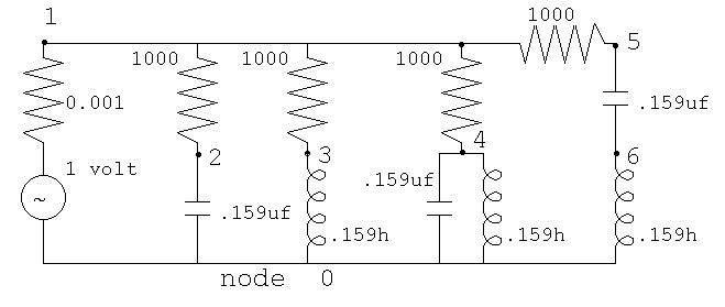 ac_plot.java simple Java plot added
ac_plot.dat capacitor, inductor and tuned circuits
ac_plot.java simple Java plot added
ac_plot.dat capacitor, inductor and tuned circuits
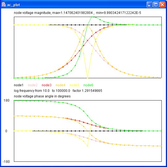 Output of java myjava.ac_plot.java < ac_plot.dat
There are systems of equations with no solutions:
eq1: 1*x + 0*y + 0*z = 2
eq2: 2*x + 0*y + 0*z = 2
eq3: 4*x - 2*y + 3*z = 5
Some may ask: What about solving |A| * |X| = |Y| for X, given A and Y
using |X| = |Y| * |A|^-1 (inverse of matrix A) ?
The reason this is not a good numerical solution is that slightly
more total error will be in the inverse |A|^-1 and then a little
more error will come from the vector times matrix multiplication.
Output of java myjava.ac_plot.java < ac_plot.dat
There are systems of equations with no solutions:
eq1: 1*x + 0*y + 0*z = 2
eq2: 2*x + 0*y + 0*z = 2
eq3: 4*x - 2*y + 3*z = 5
Some may ask: What about solving |A| * |X| = |Y| for X, given A and Y
using |X| = |Y| * |A|^-1 (inverse of matrix A) ?
The reason this is not a good numerical solution is that slightly
more total error will be in the inverse |A|^-1 and then a little
more error will come from the vector times matrix multiplication.
Matrix Inverse
The code for matrix inverse is very similar to the code for solving
simultaneous equations. Added effort is needed to find the
maximum pivot element and there must be both row and column
interchanges. An example that shows the increasing error with the
increasing size of the matrix, on a difficult matrix, is shown below.
Note that results of a 16 by 16 matrix using 64-bit IEEE Floating
point arithmetic that is ill conditioned may become useless.
inverse.f90
test_inverse.f90
test_inverse_f90.out
Extracted form test_inverse_f90.out is
initializing big matrix, n= 2 , n*n= 4
sum of error= 1.84748050191530E-16 , avg error= 4.61870125478825E-17
initializing big matrix, n= 4 , n*n= 16
sum of error= 2.19971263426544E-12 , avg error= 1.37482039641590E-13
initializing big matrix, n= 8 , n*n= 64
sum of error= 0.00000604139304982709 , avg error= 9.43967664035483E-8
initializing big matrix, n= 16 , n*n= 256
sum of error= 83.9630735209012 , avg error= 0.327980755941020
initializing big matrix, n= 32 , n*n= 1024
sum of error= 4079.56590417946 , avg error= 3.98395107830025
initializing big matrix, n= 64 , n*n= 4096
sum of error= 53735.8765782488 , avg error= 13.1191104927365
initializing big matrix, n= 128 , n*n= 16384
sum of error= 85784.2643647822 , avg error= 5.23585597929579
initializing big matrix, n= 256 , n*n= 65536
sum of error= 1097119.16168229 , avg error= 16.7407098645368
initializing big matrix, n= 512 , n*n= 262144
sum of error= 1.36281435213093E+7 , avg error= 51.9872418262837
initializing big matrix, n= 1024 , n*n= 1048576
sum of error= 1.24247404738082E+9 , avg error= 1184.91558778841
Very similar results from the C version:
inverse.c
test_inverse.c
test_inverse.out
inverse.py
test_inverse.py
test_inverse_py.out
test_inv.py numpy version
test_inv_py.out
Extracted form test_inverse.out is
initializing big matrix, n=1024, n*n=1048576
sum of error=1.24247e+09, avg error=1184.92
Inverse.rb Ruby class Inverse
test_inverse.rb Ruby test
test_inverse_rb.out Ruby output
Multiple Precision
A case study using 32-bit IEEE floating point and 50, 100, and 200
digit multiple precision are shown in Lecture 3a
Reducing the number of equation when some values are known
Later, when we study partial differential equations, we will need
cs455_l3c.shtml a process for reducing the number
of equations when we know the value of one or more elements
of the unknown vector.
Nonlinear equations and systems of nonlinear equations
are covered in Lecture 16
Really difficult, are systems of nonlinear equations that need
a solution. The following examples have many comments describing
one or more possible methods of solution:
(Later versions have fewer bugs)
simeq_newton.adb with debug printout
simeq_newton_ada.out
simeq_newton2.adb
simeq_newton2_ada.out
simeq_newton5.adb
test_simeq_newton5.adb
test_simeq_newton5_ada.out
real_arrays.ads used by above
real_arrays.adb used by above
inverse.adb used by above
equation_nl.adb with debug printout
equation_nl_ada.out
simeq_newton.f90 with debug printout
simeq_newton_f90.out
simeq_newton2.f90
simeq_newton2_f90.out
inverse.f90 used by above
udrnrt.f90 used by above
equation_nl.f90 with debug printout
equation_nl_f90.out
simeq_newton.c with debug printout
simeq_newton.out
simeq_newton2.c
simeq_newton2.out
simeq_newton3.h
simeq_newton3.c
test_simeq_newton3.c
test_simeq_newton3_c.out
simeq_newton4.h
simeq_newton4.c
test_simeq_newton4.c
test_simeq_newton4_c.out
invert.h used by above
invert.c used by above
udrnrt.h used by above
udrnrt.c used by above
equation_nl.c with debug printout
equation_nl_c.out
simeq_newton.java with debug printout
simeq_newton2.java
test_simeq_newton2.java
test_simeq_newton2_java.out
simeq_newton3.java
test_simeq_newton3.java
test_simeq_newton3.java
simeq_newton5.java
test_simeq_newton5.java
test_simeq_newton5.java
test_pde_nl.java
test_pde_nl_java.out
test_46_nl.java simple demo
test_46_nl_java.out simple demo
simeq_newton5.py3
test_pde_nl.py3 simple test
test_pde_nl_py3.out simple test
simeq_newton5.java
test_simeq_newton5.java
test_simeq_newton5_java.out
invert.java used by above
equation_nl.java with debug printout
equation_nl_java.out
inverse.java used by above
Accuracy does degrade as the relative size of solution and
matrix elements gets large. Expect similar results with any method.
This program tests 0, 1, 2, 5, ... 1E9, 2E9, 5E9, 1E10 for various n.
simeq_accuracy.c big range test
simeq_accuracy_c.out big range results
Accuracy of all methods degrades with size of matrix on random data.
Not much error for 1024 by 1024 matrix.
Errors increase at 2048 by 2048 and 4096 by 4096.
Over 10K by 10K starts to need multiple precision floating point,
see next lectures.
For your information, modern manufacturing of automobiles:
www.youtube.com/embed/8_lfxPI5ObM?rel=0
<- previous index next ->
-
CMSC 455 home page
-
Syllabus - class dates and subjects, homework dates, reading assignments
-
Homework assignments - the details
-
Projects -
-
Partial Lecture Notes, one per WEB page
-
Partial Lecture Notes, one big page for printing
-
Downloadable samples, source and executables
-
Some brief notes on Matlab
-
Some brief notes on Python
-
Some brief notes on Fortran 95
-
Some brief notes on Ada 95
-
An Ada math library (gnatmath95)
-
Finite difference approximations for derivatives
-
MATLAB examples, some ODE, some PDE
-
parallel threads examples
-
Reference pages on Taylor series, identities,
coordinate systems, differential operators
-
selected news related to numerical computation