<- previous index next ->
Go over WEB pages Lecture 1 through 29, including:
3a, 3b, 18a, 24a, 24b, 27a and 28a.
Open book, open notes
Read the instructions.
Follow the instructions, else lose points.
Read the question carefully.
Answer the question that is asked, not the question you want to answer.
Go over Quiz1 and Quiz2. Some of those questions may be reused.
Go over Lecture 9 Review, Lecture 19 Review.
Things you should know:
It is best to find working code to do the numerical computation that
you need, rather than to develop the code yourself.
Thoroughly test any numerical code you are planning to use.
Convert existing, tested, numerical code to the language of your choice.
It is usually better to convert working numerical code to the language
of your choice, rather than creating a multi language interface.
(The exception to this suggestion is LAPACK.)
Modify the interfaces as needed for your application.
Do not put trust in benchmarks that others have run. Run your own benchmarks.
It is possible for operating system code or library code to have an
error that causes incorrect time for a benchmark.
A benchmark must run long enough to avoid error due to the hardware
or software quantization of time. Ten seconds has been found acceptable
on most computers. Less that one second has been found to be bad on
a few computers.
Dead code elimination can cause a benchmark to appear to run very fast.
Using an "if" statement or "print" statement of computed variable
can prevent dead code elimination.
If you are unable to run a benchmark yourself, try to find benchmarks
that resembles what you are interested in.
It is possible to computer derivatives very accurately with high
order equations. A function is available in a few languages to
compute the required coefficients.
Derivatives can be computed for any function that can be evaluated.
By using more function evaluations, better accuracy can be obtained.
Making the step size extremely small may hurt accuracy.
A second derivative can be computed by numerically computing two
successive first derivatives. Yet, accuracy will be better when
using the formulas for second order derivatives.
More function evaluations are required in order to maintain the
same order of accuracy for each higher derivative.
Ordinary differential equations have only one independent variable.
Partial differential equations have more than one independent variable.
The "order" of a differential equation is the highest derivative in
the equation.
The "degree" of a differential equation is the highest power of
any combinations of variables and unknown solution.
The "dimension" of a differential equation is the number of
independent variables.
"initial value" problems have enough information to start
computing the solution from the initial point in every dimension.
"boundary value" problems have the solution, Dirchlet, values
given on the boundary of every dimension. The slope, Neumann,
values may also be provided.
Many specific names are given to differential equations:
"parabolic" "diffusion equation" "hyperbolic" "wave equation"
"elliptic" "Laplace's equation" "biharmonic equation" etc.
Given y=f(x) the first derivatives of f(x) may be written as
y' f' f'(x) df/dx .
For partial derivatives, given z=f(x,y) dz/dx may be written as fx,
dz/dy may be written as fy, d^3z/dx^2 dy man be written fxxy .
(and may use partial derivative symbol in place of d )
The Runge-Kutta method is a common way to compute an iterative solution,
initial value problem, to an ordinary differential equation.
Solving a system of linear equations is a common way to compute a
solution to both ordinary and partial differential equations.
Generally, boundary value problems.
The unknowns in the system of differential equations being used
to solve a differential equations are the values of the unknown
function at specific points. e.g. y(h), y(2h), y(3h), etc.
Given a fourth order ordinary differential equation with only
initial conditions, y'''' = f(x), in order to find a unique
numerical solution, values for c must be given for:
c1 = y(x0) c2 = y'(x0) c3 = y''(x0) c4 = y'''(x0)
and all the values must be at the same x0.
A method that might give reasonable results for the above equation can be:
x = x0
y = c1
yp = c2 yp is for y'
ypp = c3
yppp = c4
L: ypppp = f(x)
yppp = yppp + h * ypppp
ypp = ypp + h * yppp
yp = yp + h * ypp
y = y + h * yp this is the solution at x0+h
x = x + h loop to L: for more values.
could print or save x,y
Much of Lecture 27 and 28 were from the source code:
pde3.c A second order partial differential equation with
boundary values, two independent variables, with equal
step size, using an iterative method.
pde3_eq.c same as pde3.c with the iteration replaced by a call
to simeq and the setup of the matrix in init_matrix.
pde3b.c A similar second order partial differential equation
with boundary values, three independent variables and
each independent variable can have a unique step size
and a unique number of points to be evaluated.
pde3b_eq.c same as pde3b.c with the iteration replaced by a call
to simeq and the setup of the matrix in init_matrix.
Notice that these programs were also provided in various other
languages and looked very similar.
The problem was provided in the comments and in the code.
These "solvers" had the solution programmed in so that the method
and the code could be tested. In general the solution is not
known. The solution is computed at some specific points. If the
solution is needed at other points, then interpolation is used.
These "solvers" were based on solving a partial differential
equation that was continuous and continuously differentiable.
There are many specialized solvers for specific partial differential
equations. These lectures just covered two of the many methods
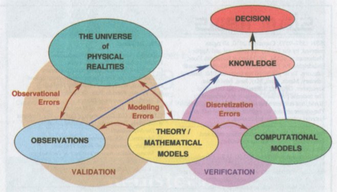
You have learned about modeling and simulation
You have worked with physical world modeling and simulation
by numerical computation. This is a valuable skill in helping
your future employer reach good decisions, as shown in the
diagram from SIAM Review.
<- previous index next ->
-
CMSC 455 home page
-
Syllabus - class dates and subjects, homework dates, reading assignments
-
Homework assignments - the details
-
Projects -
-
Partial Lecture Notes, one per WEB page
-
Partial Lecture Notes, one big page for printing
-
Downloadable samples, source and executables
-
Some brief notes on Matlab
-
Some brief notes on Python
-
Some brief notes on Fortran 95
-
Some brief notes on Ada 95
-
An Ada math library (gnatmath95)
-
Finite difference approximations for derivatives
-
MATLAB examples, some ODE, some PDE
-
parallel threads examples
-
Reference pages on Taylor series, identities,
coordinate systems, differential operators
-
selected news related to numerical computation