<- previous index next ->
Numerical differentiation can be applied to all coordinate systems.
It gets more complicated, yet a reasonable extension of Cartesian
coordinate systems. These are all partial derivatives.
The algorithms and some code shown below will be used when the
function is unknown, when we are solving partial differential
equations in non Cartesian coordinate systems.
Polar coordinates
Consider a function f(r,theta) that you can compute but do not know
a symbolic representation. To find the derivatives at a point
(r,theta) in a polar coordinate system we will use our previously
discussed "nuderiv" nonuniform Cartesian derivative function.
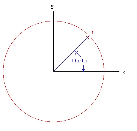 x = r * cos(Θ) r = sqrt(x^2 + y^2) 0 < r
y = r * sin(Θ) Θ = atan2(y,x) 0 ≤ θ < 2Π
^ ^
∇f(r,Θ) = r ∂f/∂r + Θ 1/r ∂f/∂Θ
∇2f(r,Θ) = 1/r ∂/∂r(r*∂f/∂r) + 1/r2 ∂2f/∂Θ2
= 2/r ∂f/∂r + ∂2f/∂r2) + 1/r2 ∂2f/∂Θ2
x = r * cos(Θ) r = sqrt(x^2 + y^2) 0 < r
y = r * sin(Θ) Θ = atan2(y,x) 0 ≤ θ < 2Π
^ ^
∇f(r,Θ) = r ∂f/∂r + Θ 1/r ∂f/∂Θ
∇2f(r,Θ) = 1/r ∂/∂r(r*∂f/∂r) + 1/r2 ∂2f/∂Θ2
= 2/r ∂f/∂r + ∂2f/∂r2) + 1/r2 ∂2f/∂Θ2
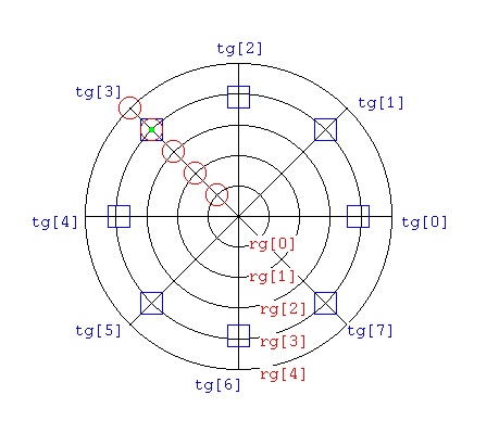 Neither radius grid "rg[]" nor theta grid "tg[]" need to be uniformly
spaced. To compute the derivatives at the green dot, (rg[3],tg[3])
Use the red circle grid points for ∂/∂r and ∂2/∂r2
Use the blue box grid points for ∂/∂Θ and ∂2/∂Θ2
The computation, in "C" language, at rg[3],tg[3] would be:
nuderiv(1, nr, 3, rg, cr); /* nr is 5 in this example */
Ur = 0.0;
for(k=0; k<nr; k++) Ur += cr[k]*f(rg[k],tg[3]); /* ∂/∂r */
nuderiv(1, nt, 3, tg, ct); /* nt is 8 in this sample */
Ut = 0.0;
for(k=0; k<nt; k++) Ut += ct[k]*f(rg[3],tg[k]); /* ∂/∂Θ */
^
nab1r = Ur /* r ∇f(r,Θ) */
^
nab1Θ = (1.0/rg[3])*Ut; /* Θ ∇f(r,Θ) */
nuderiv(2, nr, 3, rg, crr); /* nr is 5 in this example */
Urr = 0.0;
for(k=0; k<nr; k++) Urr += crr[k]*f(rg[k],tg[3]); /* ∂2/∂r2 */
nuderiv(2, nt, 3, tg, ctt); /* nt is 8 in this example */
Utt = 0.0;
for(k=0; k<nt; k++) Utt += ctt[k]*f(rg[3],tg[k]); /* ∂2/∂Θ2 */
nab2 = (2.0/rg[3])*Ur + Urr + (1.0/(rg[3]*rg[3]))*Utt; /* ∇2f(r,Θ) */
The actual code to check these equations at all grid points is:
check_polar_deriv.adb source code
check_polar_deriv_ada.out verification output
Neither radius grid "rg[]" nor theta grid "tg[]" need to be uniformly
spaced. To compute the derivatives at the green dot, (rg[3],tg[3])
Use the red circle grid points for ∂/∂r and ∂2/∂r2
Use the blue box grid points for ∂/∂Θ and ∂2/∂Θ2
The computation, in "C" language, at rg[3],tg[3] would be:
nuderiv(1, nr, 3, rg, cr); /* nr is 5 in this example */
Ur = 0.0;
for(k=0; k<nr; k++) Ur += cr[k]*f(rg[k],tg[3]); /* ∂/∂r */
nuderiv(1, nt, 3, tg, ct); /* nt is 8 in this sample */
Ut = 0.0;
for(k=0; k<nt; k++) Ut += ct[k]*f(rg[3],tg[k]); /* ∂/∂Θ */
^
nab1r = Ur /* r ∇f(r,Θ) */
^
nab1Θ = (1.0/rg[3])*Ut; /* Θ ∇f(r,Θ) */
nuderiv(2, nr, 3, rg, crr); /* nr is 5 in this example */
Urr = 0.0;
for(k=0; k<nr; k++) Urr += crr[k]*f(rg[k],tg[3]); /* ∂2/∂r2 */
nuderiv(2, nt, 3, tg, ctt); /* nt is 8 in this example */
Utt = 0.0;
for(k=0; k<nt; k++) Utt += ctt[k]*f(rg[3],tg[k]); /* ∂2/∂Θ2 */
nab2 = (2.0/rg[3])*Ur + Urr + (1.0/(rg[3]*rg[3]))*Utt; /* ∇2f(r,Θ) */
The actual code to check these equations at all grid points is:
check_polar_deriv.adb source code
check_polar_deriv_ada.out verification output
Cylindrical coordinates
Consider a function f(r,theta,z) that you can compute but do not know
a symbolic representation. To find the derivatives at a point
(r,theta,z) in a cylindrical coordinate system we will use our previously
discussed "nuderiv" nonuniform Cartesian derivative function.
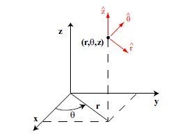 x = r * cos(Θ) r = sqrt(x^2 + y^2 + z^2) 0 < r
y = r * sin(Θ) Θ = atan2(y,x) 0 ≤ θ < 2Π
z = z z = z
^ ^ ^
∇f(r,Θ,z) = r ∂f/∂r + Θ 1/r ∂f/∂Θ + z ∂f/∂z
∇2f(r,Θ,z) = 1/r ∂/∂r(r*∂f/∂r) + 1/r2 ∂2f/∂Θ2 + ∂2f/∂z2
= 2/r ∂f/∂r + ∂2f/∂r2) + 1/r2 ∂2f/∂Θ2 + ∂2f/∂z2
x = r * cos(Θ) r = sqrt(x^2 + y^2 + z^2) 0 < r
y = r * sin(Θ) Θ = atan2(y,x) 0 ≤ θ < 2Π
z = z z = z
^ ^ ^
∇f(r,Θ,z) = r ∂f/∂r + Θ 1/r ∂f/∂Θ + z ∂f/∂z
∇2f(r,Θ,z) = 1/r ∂/∂r(r*∂f/∂r) + 1/r2 ∂2f/∂Θ2 + ∂2f/∂z2
= 2/r ∂f/∂r + ∂2f/∂r2) + 1/r2 ∂2f/∂Θ2 + ∂2f/∂z2
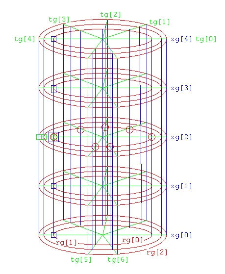 Neither radius grid "rg[]" nor theta grid "tg[]" nor the z grid "zg[]"
need to be uniformly spaced. To compute the derivatives at (rg[0],tg[4],zg[2])
Use the green box grid points for ∂/∂r; and ∂2/∂2r
Use the blue box grid points for ∂2/∂z2
Use the red circle grid points for ∂2/∂Θ2
The computation, in "C" language, would be:
nuderiv(1, nr, 0, rg, cr); /* nr is 3 in this example */
Ur = 0.0;
for(k=0; k<nr; k++) Ur += cr[k]*f(rg[k],tg[4],zg[2]); /* ∂/∂r */
nuderiv(1, nt, 4, tg, ct); /* nt is 7 in this sample */
Ut = 0.0;
for(k=0; k<nt; k++) Ut += ct[k]*f(rg[0],tg[k],zg[2]); /* ∂/∂Θ */
nuderiv(1, nz, 2, zg, cz); /* nz is 5 in this sample */
Uz = 0.0;
for(k=0; k<nz; k++) Uz += cz[k]*f(rg[0],tg[4],zg[k]); /* ∂/∂z */
^
nab1r = Ur /* r ∇f(r,Θ,z) */
^
nab1Θ = (1.0/rg[0])*Ut; /* Θ ∇f(r,&Theta,z) */
^
nab1z = Uz /* z ∇f(r,Θ,z) */
nuderiv(2, nr, 0, rg, crr); /* nr is 3 in this example */
Urr = 0.0;
for(k=0; k<nr; k++) Urr += crr[k]*f(rg[k],tg[4],zg[2]); /* ∂2/∂r2 */
nuderiv(2, nt, 4, tg, ctt); /* nt is 7 in this example */
Utt = 0.0;
for(k=0; k<nt; k++) Utt += ctt[k]*f(rg[0],tg[k],zg[2]); /* ∂2/∂Θ2 */
nuderiv(2, nz, 2, zg, czz); /* nz is 5 in this example */
Uzz = 0.0;
for(k=0; k<nz; k++) Uzz += czz[k]*f(rg[0],tg[4],zg[k]); /* ∂2/∂z2 */
nab2 = (2.0/rg[0])*Ur + Urr + (1.0/(rg[0]*rg[0]))*Utt + Uzz; /* ∇2f(r,Θ,z) */
The actual code to check these equations at all grid points is:
check_cylinder_deriv.adb source code
check_cylinder_deriv_ada.out verification output
Neither radius grid "rg[]" nor theta grid "tg[]" nor the z grid "zg[]"
need to be uniformly spaced. To compute the derivatives at (rg[0],tg[4],zg[2])
Use the green box grid points for ∂/∂r; and ∂2/∂2r
Use the blue box grid points for ∂2/∂z2
Use the red circle grid points for ∂2/∂Θ2
The computation, in "C" language, would be:
nuderiv(1, nr, 0, rg, cr); /* nr is 3 in this example */
Ur = 0.0;
for(k=0; k<nr; k++) Ur += cr[k]*f(rg[k],tg[4],zg[2]); /* ∂/∂r */
nuderiv(1, nt, 4, tg, ct); /* nt is 7 in this sample */
Ut = 0.0;
for(k=0; k<nt; k++) Ut += ct[k]*f(rg[0],tg[k],zg[2]); /* ∂/∂Θ */
nuderiv(1, nz, 2, zg, cz); /* nz is 5 in this sample */
Uz = 0.0;
for(k=0; k<nz; k++) Uz += cz[k]*f(rg[0],tg[4],zg[k]); /* ∂/∂z */
^
nab1r = Ur /* r ∇f(r,Θ,z) */
^
nab1Θ = (1.0/rg[0])*Ut; /* Θ ∇f(r,&Theta,z) */
^
nab1z = Uz /* z ∇f(r,Θ,z) */
nuderiv(2, nr, 0, rg, crr); /* nr is 3 in this example */
Urr = 0.0;
for(k=0; k<nr; k++) Urr += crr[k]*f(rg[k],tg[4],zg[2]); /* ∂2/∂r2 */
nuderiv(2, nt, 4, tg, ctt); /* nt is 7 in this example */
Utt = 0.0;
for(k=0; k<nt; k++) Utt += ctt[k]*f(rg[0],tg[k],zg[2]); /* ∂2/∂Θ2 */
nuderiv(2, nz, 2, zg, czz); /* nz is 5 in this example */
Uzz = 0.0;
for(k=0; k<nz; k++) Uzz += czz[k]*f(rg[0],tg[4],zg[k]); /* ∂2/∂z2 */
nab2 = (2.0/rg[0])*Ur + Urr + (1.0/(rg[0]*rg[0]))*Utt + Uzz; /* ∇2f(r,Θ,z) */
The actual code to check these equations at all grid points is:
check_cylinder_deriv.adb source code
check_cylinder_deriv_ada.out verification output
Spherical coordinates
interchange Φ and Θ on diagram to agree with equations
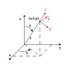 x = r * cos(Θ) * sin(Φ) r = sqrt(x^2 + y^2 + z^2) 0 < r
y = r * sin(Θ) * sin(Φ) Θ = atan2(y,x) 0 ≤ Θ < 2Π
z = r * cos(Φ) Φ = atan2(sqrt(x^2+y^2),z) 0 < Φ < Pi
^ ^ ^
∇f(r,Θ,Φ) = r ∂f/∂r + Θ 1/r sin(Φ) ∂f/∂Θ + Φ 1/r ∂f/∂φ
∇2f(r,Θ,Φ) = 1/r2 ∂/∂r(r2*∂f/∂r) + 1/(r2 sin(Φ)2) ∂2/∂Θ2f + 1/(r2 sin(Φ)) ∂/∂Φ(sin(Φ) ∂/∂f&Phi);
= 2/r ∂f/∂r + ∂2f/∂r2 + 1/(r2 sin(Φ)2) ∂2f/∂Θ2 + cos(Φ)/(r2 sin(Φ)2 ∂f/∂Φ + 1/(r2 ∂2f/∂Φ2
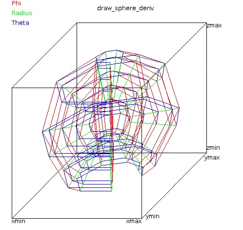
Partial derivatives in R, Theta, Phi follow their color.
All possible are shown.
x = r * cos(Θ) * sin(Φ) r = sqrt(x^2 + y^2 + z^2) 0 < r
y = r * sin(Θ) * sin(Φ) Θ = atan2(y,x) 0 ≤ Θ < 2Π
z = r * cos(Φ) Φ = atan2(sqrt(x^2+y^2),z) 0 < Φ < Pi
^ ^ ^
∇f(r,Θ,Φ) = r ∂f/∂r + Θ 1/r sin(Φ) ∂f/∂Θ + Φ 1/r ∂f/∂φ
∇2f(r,Θ,Φ) = 1/r2 ∂/∂r(r2*∂f/∂r) + 1/(r2 sin(Φ)2) ∂2/∂Θ2f + 1/(r2 sin(Φ)) ∂/∂Φ(sin(Φ) ∂/∂f&Phi);
= 2/r ∂f/∂r + ∂2f/∂r2 + 1/(r2 sin(Φ)2) ∂2f/∂Θ2 + cos(Φ)/(r2 sin(Φ)2 ∂f/∂Φ + 1/(r2 ∂2f/∂Φ2
Partial derivatives in R, Theta, Phi follow their color.
All possible are shown.
 Some "C" code to compute the derivatives at (rg[2],tg[3],zg[4])
nuderiv(2, nr, 2, rg, crr); /* nr is 3 in this example */
Urr = 0.0;
for(k=0; k<nr; k++) Urr += crr[k]*f(rg[k],tg[3],pg[4]); /* ∂2/∂r2 */
nuderiv(2, nt, 3, tg, ctt); /* nt is 7 in this example */
Utt = 0.0;
for(k=0; k<nt; k++) Utt += ctt[k]*f(rg[2],tg[k],pg[4]); /* ∂2/∂Θ2 */
nuderiv(2, np, 4, pg, cpp); /* np is 5 in this example */
Upp = 0.0;
for(k=0; k<np; k++) Upp += cpp[k]*f(rg[2],tg[3],pg[k]); /* ∂2/∂Φ2 */
nab2 = (1.0/rg[0])*Ur + Urr + (1.0/(rg[0]*rg[0]))*Utt + Uzz; /* ∇2f(r,Θ,Φ) */
The actual code to check these equations at all grid points is:
check_sphere_deriv.adb source code
check_sphere_deriv_ada.out verification output
A rather thorough test:
check_spherical_gradient.c source code
check_spherical_gradient_c.out verification output
Other checking of code and one figure came from
draw_sphere_deriv.java
draw_sphere_deriv_java.out
Many functions that do everything with spherical coordinates.
Overboard testing including Laplacian in spherical coordinates.
pde_sphere_mws.out analytic
pde_sphere.c source code
pde_sphere_c.out output
Some "C" code to compute the derivatives at (rg[2],tg[3],zg[4])
nuderiv(2, nr, 2, rg, crr); /* nr is 3 in this example */
Urr = 0.0;
for(k=0; k<nr; k++) Urr += crr[k]*f(rg[k],tg[3],pg[4]); /* ∂2/∂r2 */
nuderiv(2, nt, 3, tg, ctt); /* nt is 7 in this example */
Utt = 0.0;
for(k=0; k<nt; k++) Utt += ctt[k]*f(rg[2],tg[k],pg[4]); /* ∂2/∂Θ2 */
nuderiv(2, np, 4, pg, cpp); /* np is 5 in this example */
Upp = 0.0;
for(k=0; k<np; k++) Upp += cpp[k]*f(rg[2],tg[3],pg[k]); /* ∂2/∂Φ2 */
nab2 = (1.0/rg[0])*Ur + Urr + (1.0/(rg[0]*rg[0]))*Utt + Uzz; /* ∇2f(r,Θ,Φ) */
The actual code to check these equations at all grid points is:
check_sphere_deriv.adb source code
check_sphere_deriv_ada.out verification output
A rather thorough test:
check_spherical_gradient.c source code
check_spherical_gradient_c.out verification output
Other checking of code and one figure came from
draw_sphere_deriv.java
draw_sphere_deriv_java.out
Many functions that do everything with spherical coordinates.
Overboard testing including Laplacian in spherical coordinates.
pde_sphere_mws.out analytic
pde_sphere.c source code
pde_sphere_c.out output
<- previous index next ->
-
CMSC 455 home page
-
Syllabus - class dates and subjects, homework dates, reading assignments
-
Homework assignments - the details
-
Projects -
-
Partial Lecture Notes, one per WEB page
-
Partial Lecture Notes, one big page for printing
-
Downloadable samples, source and executables
-
Some brief notes on Matlab
-
Some brief notes on Python
-
Some brief notes on Fortran 95
-
Some brief notes on Ada 95
-
An Ada math library (gnatmath95)
-
Finite difference approximations for derivatives
-
MATLAB examples, some ODE, some PDE
-
parallel threads examples
-
Reference pages on Taylor series, identities,
coordinate systems, differential operators
-
selected news related to numerical computation