<- previous index next ->
Sound, voice, music, etc. can be in many compressed formats in
many file types, such as .wav .mp3 .aac .avi .mka .mpeg .vox ...
If your computer has a speaker and software, you can hear sound files.
On almost all browsers, click and hear sound files.
On Ubuntu programs aplay, Rythmbox, and some languages provide
for listening to sound files. There are a few programs that can be
downloaded that convert some type of sound file to another type
of sound file. 30,000 volume samples per second is common.
sudo apt install aplay
We will read a sound file, volume data at very small
time intervals, use FFT to get frequency domain.
Modify the frequency domain, IFFT to get volume and convert
to a .wav file.
A basic Fourier transform can convert a function in the time domain
to a function in the frequency domain. For example, consider a sound
wave where the amplitude is varying with time. We can use a discrete
Fourier transform on the sound wave and get the frequency spectrum.
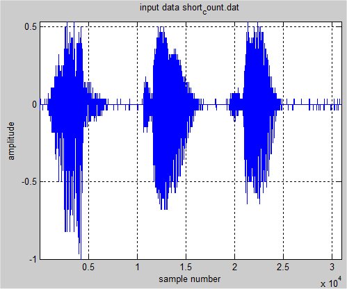
This is short_count.wav one, two, three
short_count.wav
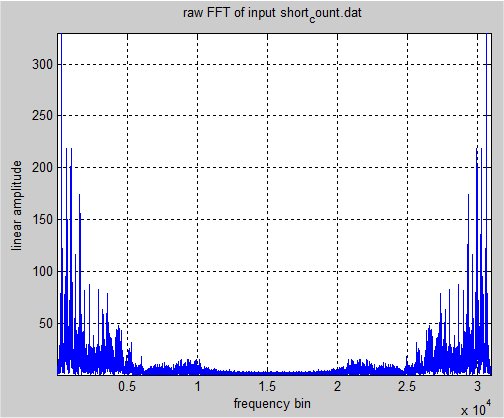
 The basic FFT plotting the magnitude of about 31,000 bins
has zero frequency on left, highest frequency in middle,
and back to lowest frequency on right:
The basic FFT plotting the magnitude of about 31,000 bins
has zero frequency on left, highest frequency in middle,
and back to lowest frequency on right:
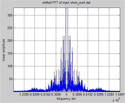
 Using fftshift to center the zero frequency:
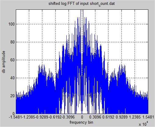
 Then taking the log of the amplitude is typical
when plotting a spectrum:
Then taking the log of the amplitude is typical
when plotting a spectrum:
 Above made using:
plot_fft.m reads .dat amplitudes
wav_to_dat.c make .dat from .wav
cat.wav, sound file, was converted cat.dat, amplitude data file
cat.wav sound
cat.dat amplitude in 18,814 time steps
Of course there is an inverse Fourier transform that converts
the frequency spectrum back to the time domain.
The spectrum of F(t)=sin(2 Pi f t) t=0..1 is a single frequency f.
The discrete transform assumes the function is repeated for all t.
The amplitude values must be sampled at equal time increments for
the spectrum to be valid. The maximum frequency that can be
computed, called the Nyquist Frequency, is one half the sampling rate.
Sampling at 10,000 samples per second has maximum frequency of 5kHz.
It turns out that a signal at some frequency has an amplitude and
a phase, or an in-phase and quadrature value. The convenient
implementation is to consider these values as complex numbers.
It turns out that some input can be collected as complex values and
thus most implementations of the FFT take an array of complex numbers
as input and produce the same size array of complex numbers as output.
For technical reasons, a simple FFT requires the size of the input
and output must be a power of 2. Special versions of the FFT as found in
FFTW the fastest Fourier transform in the west
handle arbitrary sizes. We just pad out our input data with zeros to make
the size of the array a power of 2.
Fourier transforms have many other uses such as image filtering and
pattern matching, convolution and understanding modulation.
A few, non fast, programs that compute Fourier Series coefficients for
unequally spaced samples, read from a file, are:
fourier.c
fourier.java
sin(2x) data sin2.dat
test on sine2.dat fourier_java.out
More detail of the basic Fourier transforms and series,
both continuous and discrete is fourier.pdf
square_wave_gen.c using series
square_wave_gen_c.out cos and sin
There are many many implementations of the FFT, the n log_2 n
complexity method of computing the discrete Fourier transform.
Two of the many methods are shown below.
One method has the coefficients precomputed in the source code.
A second method computes the coefficients as they are needed.
Precomputed constants for each size FFT
fft16.c fft16.adb
fft32.c fft32.adb
fft64.c fft64.adb
fft128.c fft128.adb
fft256.c fft256.adb
fft512.c fft512.adb
fft1024.c fft1024.adb
fft2048.c fft2048.adb
fft4096.c fft4096.adb
Precomputed constants of each size inverse FFT
ifft16.c ifft16.adb
ifft32.c ifft32.adb
ifft64.c ifft64.adb
ifft128.c ifft128.adb
ifft256.c ifft256.adb
ifft512.c ifft512.adb
ifft1024.c ifft1024.adb
ifft2048.c ifft2048.adb
ifft4096.c ifft4096.adb
Header file and timing program
fftc.h
fft_time.c fft_time.adb
fft_time_c.out fft_time_ada.out
A more general program that can compute the fft and inverse fft for
an n that is a power of two is:
fft.h
fft.c
fftest.c
fftin.dat binary data
fftin.out binary data
A more general program for the FFT of large data in Java is:
Cxfft.java
read_wav.java reads and writes .wav
read_wave_java.out output
these may be combined for use in HW5.
fft_wav.java transform and inverse
fft_frame.java with a very crude frequency plot
Above made using:
plot_fft.m reads .dat amplitudes
wav_to_dat.c make .dat from .wav
cat.wav, sound file, was converted cat.dat, amplitude data file
cat.wav sound
cat.dat amplitude in 18,814 time steps
Of course there is an inverse Fourier transform that converts
the frequency spectrum back to the time domain.
The spectrum of F(t)=sin(2 Pi f t) t=0..1 is a single frequency f.
The discrete transform assumes the function is repeated for all t.
The amplitude values must be sampled at equal time increments for
the spectrum to be valid. The maximum frequency that can be
computed, called the Nyquist Frequency, is one half the sampling rate.
Sampling at 10,000 samples per second has maximum frequency of 5kHz.
It turns out that a signal at some frequency has an amplitude and
a phase, or an in-phase and quadrature value. The convenient
implementation is to consider these values as complex numbers.
It turns out that some input can be collected as complex values and
thus most implementations of the FFT take an array of complex numbers
as input and produce the same size array of complex numbers as output.
For technical reasons, a simple FFT requires the size of the input
and output must be a power of 2. Special versions of the FFT as found in
FFTW the fastest Fourier transform in the west
handle arbitrary sizes. We just pad out our input data with zeros to make
the size of the array a power of 2.
Fourier transforms have many other uses such as image filtering and
pattern matching, convolution and understanding modulation.
A few, non fast, programs that compute Fourier Series coefficients for
unequally spaced samples, read from a file, are:
fourier.c
fourier.java
sin(2x) data sin2.dat
test on sine2.dat fourier_java.out
More detail of the basic Fourier transforms and series,
both continuous and discrete is fourier.pdf
square_wave_gen.c using series
square_wave_gen_c.out cos and sin
There are many many implementations of the FFT, the n log_2 n
complexity method of computing the discrete Fourier transform.
Two of the many methods are shown below.
One method has the coefficients precomputed in the source code.
A second method computes the coefficients as they are needed.
Precomputed constants for each size FFT
fft16.c fft16.adb
fft32.c fft32.adb
fft64.c fft64.adb
fft128.c fft128.adb
fft256.c fft256.adb
fft512.c fft512.adb
fft1024.c fft1024.adb
fft2048.c fft2048.adb
fft4096.c fft4096.adb
Precomputed constants of each size inverse FFT
ifft16.c ifft16.adb
ifft32.c ifft32.adb
ifft64.c ifft64.adb
ifft128.c ifft128.adb
ifft256.c ifft256.adb
ifft512.c ifft512.adb
ifft1024.c ifft1024.adb
ifft2048.c ifft2048.adb
ifft4096.c ifft4096.adb
Header file and timing program
fftc.h
fft_time.c fft_time.adb
fft_time_c.out fft_time_ada.out
A more general program that can compute the fft and inverse fft for
an n that is a power of two is:
fft.h
fft.c
fftest.c
fftin.dat binary data
fftin.out binary data
A more general program for the FFT of large data in Java is:
Cxfft.java
read_wav.java reads and writes .wav
read_wave_java.out output
these may be combined for use in HW5.
fft_wav.java transform and inverse
fft_frame.java with a very crude frequency plot
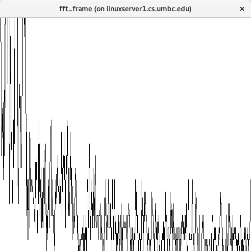 very crude frequency plot
For Matlab, fft_wav.m may be useful for HW5
fft_wav.m transform and inverse, frequency plot
Another version in "C" and Java, the Java demonstrates convolution
fftd.h
fftd.c
test_fft.c
test_fft_c.out
Cxfft.java
TestCxfft.java
TestCxfft.out
Python using downloaded numpy has fft
testfft.py
testfft.out
fftwav.py3
fftwav.py3_out
write_ran_wav.py3
plotwav.py3
print_afile.py3
MatLab has fft as well as almost every other function
test_fft.m
test_fft_m.out
test_fft2.m
test_fft2_m.out
In order to get better accuracy on predicted coefficients
for square wave, triangle wave and saw tooth wave, 1024 points.
The series are shown as comments in the code.
Also shown, is the anti aliasing and normalization needed to
get the coefficients for the Fourier series.
test_fft_big.c
test_fft_big_c.out
very crude frequency plot
For Matlab, fft_wav.m may be useful for HW5
fft_wav.m transform and inverse, frequency plot
Another version in "C" and Java, the Java demonstrates convolution
fftd.h
fftd.c
test_fft.c
test_fft_c.out
Cxfft.java
TestCxfft.java
TestCxfft.out
Python using downloaded numpy has fft
testfft.py
testfft.out
fftwav.py3
fftwav.py3_out
write_ran_wav.py3
plotwav.py3
print_afile.py3
MatLab has fft as well as almost every other function
test_fft.m
test_fft_m.out
test_fft2.m
test_fft2_m.out
In order to get better accuracy on predicted coefficients
for square wave, triangle wave and saw tooth wave, 1024 points.
The series are shown as comments in the code.
Also shown, is the anti aliasing and normalization needed to
get the coefficients for the Fourier series.
test_fft_big.c
test_fft_big_c.out
Reading and Writing .wav files for HW5
Here is a program that just reads a .wav file and writes a copy,
and does a little printing. This with extensions can be the basis
of Homework 5. fftwav.py3 , fft1_wav.c , You may modify
to suit your desires. These only work for single channel, 8 bit
per sample PCM .wav files. (not all the .wav files listed below)
Note: sound does not work from a remote computer, e.g. ssh
Some programs require special libraries or operating systems.
read_wav.c
read_wav.out
train1.wav
short_count.wav
rocky4.wav
cat.wav
Splitting out read and write wav:
rw_wav.h
rw_wav.c
test_rw_wav.c
test_rw_wav.out
And here are three .wav files from very small to larger for testing:
ok.wav
train.wav
roll.wav
fft1t.wav
short_count.wav
fft1c.wav
Suppose you wanted to compute a sound. Here is a generator for
a simple sine wave. It sounds cruddy.
sine_wav.c
sine_wav.out
sine.wav
Computing FFT of a .wav file for HW5
For the homework, one example using a 64 point FFT and just doing
the transform and inverse transform, essentially no change, is
fft1_wav.c
fft1_wav.out
trainf.wav
rockey2.wav
count_out.wav
trainf2.wav experiment
Hopefully you can find some more interesting .wav files.
P.S. When using MediaPlayer or QuickTime be sure to close the
file before trying to rewrite it.
Your web browser can usually play .wav files.
Use file:/// path to your directory /xxx.wav
In Java, ClipPlayer.java reads and
plays .wav and other files. The driver program is ClipPlayerTest.java
In Python, M$ only, with the WX graphics available, play .wav files with
sound.py
or on linux
linux_sound.py
rocky4.wav
In MatLab play .wav, old wave replaced by audio,
must be on local computer with speaker.
waveplay.m
short_count.wav
Im MatLab play .dat files that have a value for each
sample.
soundplay.m
short_count.dat
For students running Ubuntu, this sequence of "C" programs
demonstrate direct use of playing sampled amplitude sound.
These do not require generating a .wav or other type sound file.
pcm_min.c
pcm_sin.c
pcm_dat.c
Makefile_sound
short_count.dat
long_count.dat
You may modify any of these to suit your needs.
An interactive WEB site with with a few functions and their spectrum is
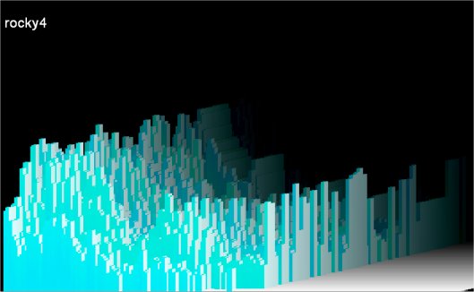
heliso.tripod.com/java_hls/gccs/spectrum1.htm
Here is Rocky speaking and the dynamic spectrum
rocky4.wav
This needs modifications for 2 channel and 16 bits per sample.
 Now you can do homework 5
You may not have your own web page activated to play your .wav files:
do these commands:
cp my.vav ~/pub/www/
cd ~/pub/www/
chmod go+rx my.wav
cd ..
chmod go+rx www
cd ~
you are back in your login directory, and from home you can
http://www.gl.umbc.edu/~your-user-id
then click on my.wav
optional plots of FFT's using Python and C with gnuplot
plot_fft_py.html
plot_fft_c.html
Now sound in db:
cs455_l18a.html
Then FFT to determine material, molecules.
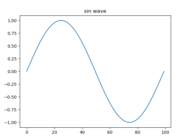
Making spectrum to get wave shape, Gibb to square wave
wave = sum (1.0/g)*sin(g*x) g = 1, 3, 5, 7, 9, ... 75
plot_gibb.py3 source code
plot_gibb_py3.out output
Plotted results:
Now you can do homework 5
You may not have your own web page activated to play your .wav files:
do these commands:
cp my.vav ~/pub/www/
cd ~/pub/www/
chmod go+rx my.wav
cd ..
chmod go+rx www
cd ~
you are back in your login directory, and from home you can
http://www.gl.umbc.edu/~your-user-id
then click on my.wav
optional plots of FFT's using Python and C with gnuplot
plot_fft_py.html
plot_fft_c.html
Now sound in db:
cs455_l18a.html
Then FFT to determine material, molecules.
Making spectrum to get wave shape, Gibb to square wave
wave = sum (1.0/g)*sin(g*x) g = 1, 3, 5, 7, 9, ... 75
plot_gibb.py3 source code
plot_gibb_py3.out output
Plotted results:
 plot_gibb_1.png
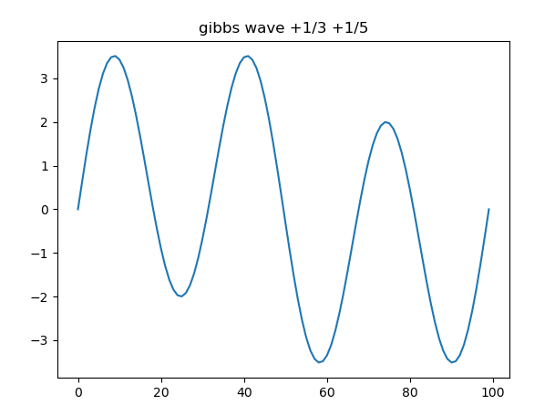 plot_gibb_3.png
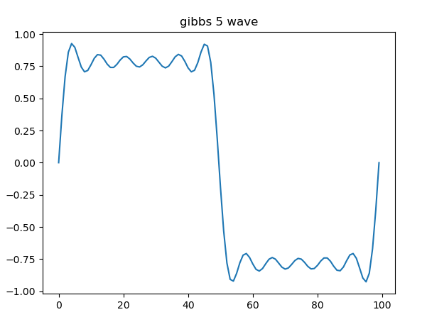 plot_gibb_5.png
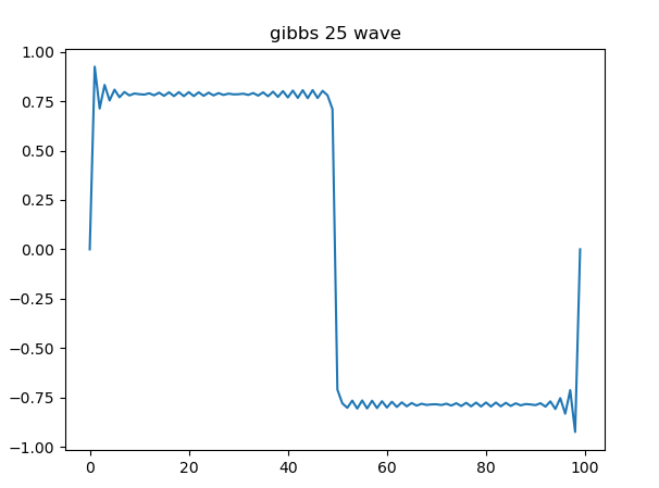 plot_gibb_25.png
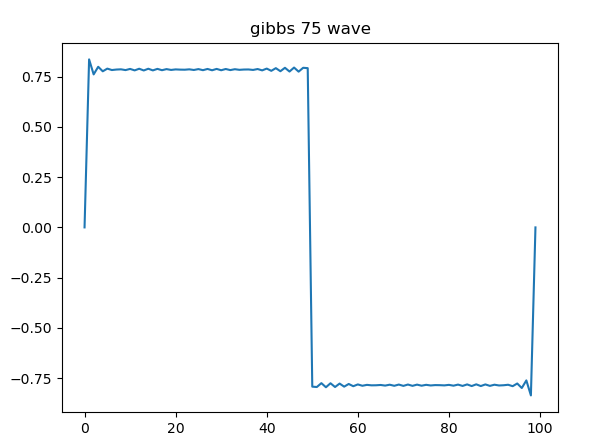 plot_gibb_75.png
<- previous index next ->
-
CMSC 455 home page
-
Syllabus - class dates and subjects, homework dates, reading assignments
-
Homework assignments - the details
-
Projects -
-
Partial Lecture Notes, one per WEB page
-
Partial Lecture Notes, one big page for printing
-
Downloadable samples, source and executables
-
Some brief notes on Matlab
-
Some brief notes on Python
-
Some brief notes on Fortran 95
-
Some brief notes on Ada 95
-
An Ada math library (gnatmath95)
-
Finite difference approximations for derivatives
-
MATLAB examples, some ODE, some PDE
-
parallel threads examples
-
Reference pages on Taylor series, identities,
coordinate systems, differential operators
-
selected news related to numerical computation