<- previous index next ->
Eigenvalue and Eigenvector computation may be the most prolific for
special case numerical computation. Considering the size and speed
of modern computers, I use a numerical solution for a general
complex matrix. Thus, I do not have to worry about the constraints
on the matrix (is it numerically positive definite?)
The eigenvalues of a matrix with only real elements may be complex.
| 2.0 -2.0 |
| 1.0 0.0 | has eigenvalues 1+i and 1-i
Thus, computing eigenvalues needs to use complex arithmetic.
This type of numerical algorithm, you do not want to develop yourself.
The technique is to find a working numerical code, test it yourself,
then adapt the code to your needs, possibly converting the code to
a different language.
Eigenvalues have application in the solution of some physics problems.
They are also used in some solutions of differential equations.
Some statistical analysis uses eigenvalues. Sometimes only the
largest or second largest eigenvalues are important.
My interest comes from the vast types of testing that can, and should,
be performed on any code that claims to compute eigenvalues and
eigenvectors. Thorough testing of any numeric code you are going
to use is essential.
Information about eigenvalues, e (no lambda in plain ASCII)
and eigenvectors, v, for arbitrary n by n complex matrix A.
There are exactly n eigenvalues (some may have multiplicity greater than 1)
For every eigenvalue there is a corresponding eigenvector.
For eigenvalues with multiplicity greater than 1,
each has a unique eigenvector.
The set of n eigenvectors form a basis, they are all mutually orthogonal.
(The dot product of any pair of eigenvectors is zero.)
View this page in a fixed width font, else the matrices are shambles.
Vertical bars, | |, in this lecture is not absolute value,
it means vector or matrix
| 1 0 0 |
det|A-eI| = 0 defines e, where I is an n by n identity matrix | 0 1 0 |
zero except 1 on the diagonal | 0 0 1 |
(n e's for n by n A)
For a 3 by 3 matrix A:
| a11-e a12 a13 |
det| a21 a22-e a23 | = (a11-e)*(a22-e)*(a33-e)+a12*a23*a31+a13*a32*a21-
| a31 a32 a33-e | a31*(a22-e)*a13-a21*a12*(a33-e)-a32*a23*(a11-e)
Writing out the above determinant gives the "Characteristic Equation"
of the matrix A.
Combining terms gives e^n + c_n-1 * e^n-1 + ... + c_2 * e^2 + c_1 * e + c_0 = 0
(Divide through by c_n, to have exactly n unknown coefficients 0..n-1).
(Special case because of " = 0 " )
There are exactly n roots for an nth order polynomial and the
n roots of the characteristic equation are the n eigenvalues.
The relation between each eigenvalue and its corresponding eigenvector is
Av = ev where |v| is non zero.
Typically, we require the length of v to be 1.
Given a matrix A and a non singular matrix P and P inverse p^-1
B = P A P^-1 the matrix B has the same eigenvalues as matrix A.
The eigenvectors may be different.
B is a similarity transform of A.
The diagonal elements of a diagonal matrix are the eigenvalues of the matrix.
| a11 0 0 0 |
| 0 a22 0 0 |
| 0 0 a33 0 | has eigenvalues a11, a22, a33, a44 and
| 0 0 0 a44 |
corresponding eigenvectors
v1=|1 0 0 0| v2=|0 1 0 0| v3=|0 0 1 0| v4=|0 0 0 1|
Notice that the eigenvectors are not necessarily unique and may be
scaled by an arbitrary, non zero, constant. Normalizing the length
of each eigenvector to 1.0 is common.
The eigenvalues of a 2 by 2 matrix are easily computed as the roots
of a second order equation.
det| a11-e a12 |=0 or (a11-e)*(a22-e) - a12*a21 = 0 or
| a21 a22-e |
e^2 - (a11+a22) e + (a11*a22-a12*a21) = 0
Let a=1, b=-(a11+a22), c= (a11*a22-a12*a21)
then e = (-b +/- sqrt(b^2-4*a*c)/2*a computes the two eigenvalues.
The roots and thus the eigenvalues may be complex.
Note that a matrix with all real coefficients may have complex eigenvalues
and or complex eigenvectors:
A= | 1 -1 | Lambda= 1 + i vec x= | i -1 |
| 1 1 | Lambda= 1 - i vec x= |-i 1 |
Computing the characteristic equation is usually not a good way
to compute eigenvalues for n greater than 4 or 5.
It becomes difficult to compute the coefficients of the characteristic
equation accurately and it is also difficult to compute the roots accurately.
Note that given a high order polynomial, a matrix can be set up from
the coefficients such that the eigenvalues of the matrix are the roots
of the polynomial. x^4 + c_3 x^3 + c_2 x^2 + c_1 x + c_0 = 0
| -c_3 -c_2 -c_1 -c_0 | where c_4 of the polynomial is 1.0
| 1 0 0 0 |
| 0 1 0 0 |
| 0 0 1 0 |
Thus, if you have code that can find eigenvalues, you have code
that can find roots of a polynomial. Not the most efficient method.
matrixfromroots.py3
matrixfromroots_py3.out
The maximum value of the sum of the absolute values of each row and column
is a upper bound on the absolute value of the largest eigenvalue.
This maximum value is typically called the L1 norm of the matrix.
Test, get biggest absolute value of every row and column, then
compare to absolute value of every eigenvalue.
Scaling a matrix by multiplying every element by a constant causes
every eigenvalue to be multiplied by that constant. The constant may
be less than one, thus dividing works the same.
Usually test times 2.
The eigenvalues of the inverse of a matrix are the reciprocals
of the eigenvalues of the original matrix. They may be printed
in a different order. Harder test.
The eigenvectors of the inverse of a matrix are the same as
the eigenvectors of the matrix. They may differ in order and sign.
Sample test on 3 by 3 matrix, real and complex:
eigen3q.m
eigen3q_m.out
eigen3r.m
eigen3r_m.out
A matrix with all elements equal has one eigenvalue equal to
the sum of a row and all other eigenvalues equal to zero.
The eigenvectors are typically chosen as the unit vectors.
| 0 0 0 |
A = | 0 0 0 | has three eigenvalues, all equal to zero
| 0 0 0 |
| 1 1 1 | | 2 2 2 2 |
| 1 1 1 | | 2 2 2 2 | 1 has eigenvalues 0, 0, 3
| 1 1 1 | | 2 2 2 2 | 2 has eigenvalues 0, 0, 0, 8
| 2 2 2 2 | in general n-1 zeros and a row sum
Each row that increases the singularity of a matrix, increases
the multiplicity of some eigenvalue.
The trace of a matrix is the sum of the diagonal elements.
The trace of a matrix is equal to the sum of the eigenvalues.
Another test, easy one.
In order to keep the same eigenvalues, interchanging two rows
of a matrix, then requires interchanging the corresponding two columns.
The eigenvectors will probably be different.
Sample test in Matlab showing the above
eigen10.m source code
eigen10_m.out results
Testing code that claims to compute eigenvalues
Testing a program that claims to compute eigenvalues and eigenvectors
is interesting because there are many possible tests. All should be
used.
Given A is an n by n complex matrix (that may have all real elements),
using IEEE 64-bit floating point and good algorithms:
1) Evaluate the determinant det|A-eI| for each eigenvalue, e.
The result should be near zero. 10^-9 or smaller can be expected
when A is small and eigenvalues are about the same magnitude.
2) Evaluate each eigenvalue with its corresponding eigenvector.
Av-ev should be a vector with all elements near zero.
Typically check the magnitude of the largest element.
10^-9 or smaller can be expected when A is small.
3) Compute the dot product of every pair of eigenvectors
and check for near zero. Eigenvectors should have length 1.0
4) Compute the trace of A and subtract the sum of the eigenvalues.
The result should be near zero. The trace of a matrix is the
sum of the diagonal elements of the matrix.
5) Compute the maximum of the sum of the absolute values of each
row and column of A. Check that the absolute value of every
eigenvalue is less that or equal this maximum.
6) Create a matrix from a polynomial and check that eigenvalues
are the roots of the polynomial.
7) Create a similar matrix B = P * A * P^-1 and check that
eigenvalues of B are same as eigenvalues of A.
Test cases may use random numbers or selected
real or complex numbers.
Generating test matrices to be used for testing.
1) Try matrices with n=1,2,3 first.
All zero matrix, all eigenvalues zero and eigenvectors should
be the unit basis vectors. If the length of the eigenvectors
is not 1.0, then you have to normalize them.
2) Try diagonal matrices with n=1,2,3,4
Typically put 1, 2, 3, 4 on the diagonal to make it easy to
check the values of the computed eigenvalues.
3) Generate a random n by n matrix, P, with real and imaginary values.
Compute P inverse, P^-1.
Compute matrix B = P A P^-1 for the A matrices in 2)
The eigenvalues of B should be the same as the eigenvalues of A,
yet the eigenvectors may be different.
4) Randomly interchange some rows and corresponding columns of B.
The eigenvalues should be the same yet the eigenvectors
may be different.
5) Choose a set of values, typically complex values e1, e2, ..., en.
Compute the polynomial that has those roots
(x-e1)*(x-e2)*...*(x-en) and convert to the form
x^n + c_n-1 x^n-1 + ... c_2 x^2 + c_1 x + c_0
Create the matrix n by n with the first row being negative c's
and the subdiagonal being 1's.
| -c_n-1 ... -c_2 -c_1 -c_0 |
| 1 0 0 0 |
...
| 0 0 0 0 |
| 0 1 0 0 |
| 0 0 1 0 |
The eigenvalues should be e1, e2, ..., en
Then do a similarity transform with a random matrix
and check that the same eigenvalues are computed.
Yes, this is a lot of testing, yet once coded, it can be used
for that "newer and better" version the "used software salesman"
is trying to sell you.
Sample code in several languages
Now, look at some code that computes eigenvalues and eigenvectors
and the associated test code.
First, MatLab
% eigen.m demonstrate eigenvalues in MatLab
format compact
e1=1; % desired eigenvalues
e2=2;
e3=3;
e4=4;
P=poly([e1 e2 e3 e4]) % make polynomial from roots
r=roots(P) % check that roots come back
A=zeros(4);
A(1,1)=-P(2); % build matrix A
A(1,2)=-P(3);
A(1,3)=-P(4);
A(1,4)=-P(5);
A(2,1)=1;
A(3,2)=1;
A(4,3)=1
[v e]=eig(A) % compute eigenvectors and eigenvalues
I=eye(4); % identity matrix
for i=1:4
z1=det(A-I.*e(i,i)) % should be near zero
end
for i=1:4
z2=A*v(:,i)-e(i,i)*v(:,i) % note columns, near zero
end
z3=trace(A)-trace(e) % should be near zero
% annotated output
%
%P =
% 1 -10 35 -50 24
%r =
% 4.0000 these should be eigenvalues
% 3.0000
% 2.0000
% 1.0000
%A =
% 10 -35 50 -24 polynomial coefficients
% 1 0 0 0
% 0 1 0 0
% 0 0 1 0
%v =
% 0.9683 0.9429 0.8677 0.5000 eigenvectors
% 0.2421 0.3143 0.4339 0.5000 are
% 0.0605 0.1048 0.2169 0.5000 columns
% 0.0151 0.0349 0.1085 0.5000
%e =
% 4.0000 0 0 0 eigenvalues
% 0 3.0000 0 0 as diagonal
% 0 0 2.0000 0 of the matrix
% 0 0 0 1.0000
%z1 =
% 1.1280e-13 i=1 first eigenvalue
%z1 =
% 5.0626e-14
%z1 =
% 1.3101e-14
%z1 =
% 2.6645e-15
%z2 =
% 1.0e-14 * note multiplier i=1
% -0.4441
% -0.1110
% -0.0333
% -0.0035
%z2 =
% 1.0e-14 *
% -0.4441
% -0.1554
% -0.0444
% -0.0042
%z2 =
% 1.0e-14 *
% -0.7994
% -0.2776
% -0.0833
% -0.0028
%z2 =
% 1.0e-13 *
% -0.3103
% -0.0600
% -0.0122
% -0.0033
%z3 =
% -7.1054e-15 trace check
Now very similar code in MatLab using complex eigenvalues.
A similarity transform is applied and scaling is applied.
One eigenvalue check is now accurate to about 10^-7.
(Matrix initialized with complex values 4+1i, ...)
eigen2.m
eigen2_m.out
Using complex similarity transform:
eigen3.m
eigen3_m.out
Using special cases:
eigen9.m
eigen9_m.out
Note that the MatLab help on "eig" says they use the
LAPACK routines. The next lecture covers some LAPACK.
Now python code, built in, for complex eigenvalues,
and also SVD and QR.
complex.py3
complex_py3.out
test_qrd.py
test_qrd_py.out
test_qrd.java
test_qrd_java.out
Singular Value Decomposition SVD is similar to eigenvalues.
Given a matrix A, the singular values are the positive real
square root of the eigenvalues of A A^t A times transpose of A.
(conjugate transpose if A has complex values)
(A does not need to be square)
The result U, S, V^t are computed with diagonal of S being
the singular values and A = U S V^t with columns of V transpose
being vectors.
Singular values are always returned largest first down to
smallest last. If the eigenvalues of A happen to be real and
positive, then the eigenvalues and singular values are the same.
example SVD test in matlab
test_svd.m
test_svd_m.out
example SVD test in Python, both eig and svd
test_svd.py
test_svd_py.out
test_svd0.py3
test_svd0_py3.out
A Fortran program to compute eigenvalues and eigenvectors from
TOMS, ACM Transactions on Mathematical Software, algorithm 535:
535.for
535.dat
535.out
535_roots.out
535_d.out
535_double.for double precision
535.dat
535_double_f.out
535_2.dat
535_2.out
535b.dat
535b.out
535_double.f90 just ! for C
535.rand
535_rand_f90.out
535.ranA
535_ranA_f90.out
A Java program to compute eigenvalues and eigenvectors is:
Eigen2.java
TestEigen2.java
TestEigen2.out
ruby programs to compute eigenvalues and eigenvectors using ruby Matrix:
eigen2.rb source code
eigen2_rb.out output
test_eigen1.rb source code
test_eigen1_rb.out output
test_eigen2.rb source code
test_eigen2_rb.out output
An Ada program to compute eigenvalues and eigenvectors is:
generic_complex_eigenvalues.ada
test_generic_complex_eigenvalues.ada
generic_complex_eigen_check.ada
A fortran program, from LAPACK, to compute SVD.
Note: V is conjugate transpose of eigen vectors.
cgesvd.f
A rather limited use eigenvalue computation method is the
power method. It works sometimes and may require hundreds
of iterations. The following code shows that is can work
for finding the largest eigenvalue of a small real matrix.
eigen_power.c
eigen_power_c.out
The general eigen problem is A*v = e*B*v
Checks are also det|V|=0 det|(B^-1*A)-eI|=0
Each eigenvalue e has an eigenvector v as a column of V.
A rather quick and dirty translation of 535_double.for to Ada:
test_eigen.adb
cxhes.adb Hessenberg reduction
cxval.adb compute eigenvalues
cxvec.adb compute eigenvectors
cxcheck.adb compute residual
eigdet.adb check eigenvalues
evalvec.adb check eigenvectors
cxinverse.adb invert matrix
complex_arrays.ads
complex_arrays.adb
real_arrays.ads
real_arrays.adb
test_eigen_ada.out
Built command gnatmake test_eigen.adb
Run command test_eigen > test_eigen_ada.out
rmatin.adb read 535_double.f90 data
test_535_eigen.adb
test_535_eigen_ada.out 535.dat
test_535b_eigen_ada.out 535b.dat
test_535_2_eigen_ada.out 535_2.dat
test_535_x12_eigen_ada.out 535_x12_1.dat
eigen10.m
eigen10_m.out
test_vpa.m
test_vpa_m.out
In aircraft design, there are stability questions that can be
answered using eigenvalue computations. In Matlab, you can
draw objects, such as this crude airplane, as well as doing
numerical computation.
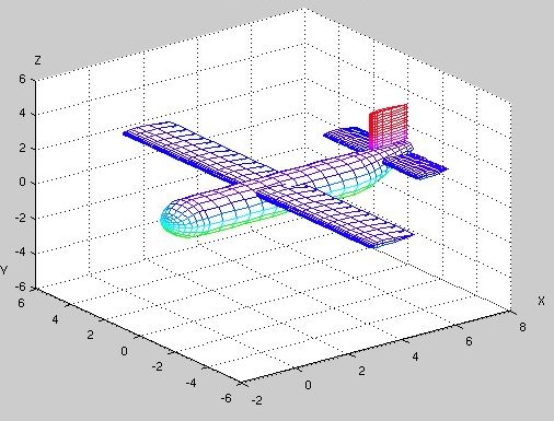 drawn by plane.m
wing_2d.m
rotx_.m
roty_.m
rotz_.m
drawn by plane.m
wing_2d.m
rotx_.m
roty_.m
rotz_.m
OK, long lecture, extra topic:
Generating random numbers, valuable for some testing.
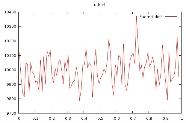
First we generate uniformly distributed random numbers in
the range 0.0 to 1.0. A uniform distribution should have
roughly the same number of values in each range, bin.
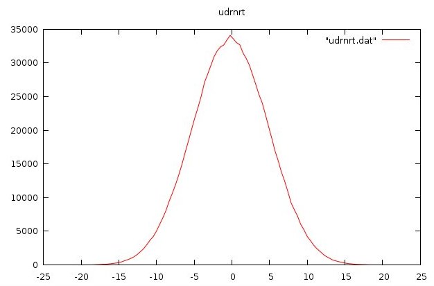
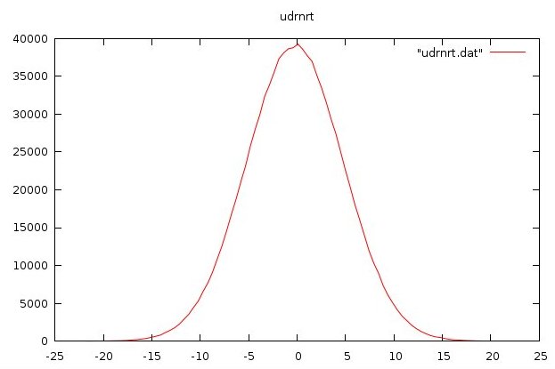
Gaussian or Normal distributions should have roughly
a bell shaped curve, based on a given mean and sigma.
Sigma is the standard deviation. Sigma squared is the variance.
udrnrt.h three generators
udrnrt.c three generators code
plot_udrnrt.c test_program
plot_udrnrt1.out udrnrt output and plot
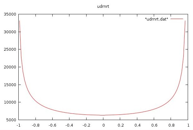
 2.0*udrnrt()-1.0 output, -1.0 to 1.0
plot_udrnrt2.out gauss output and plot
2.0*udrnrt()-1.0 output, -1.0 to 1.0
plot_udrnrt2.out gauss output and plot
 plot_udrnrt3.out gauss output and plot
 plot_udrnrt4.out sine wave output and plot
 test_rand.py uniform and gauss plot
test_rand.py3 uniform and gauss plot
test_rand.py uniform and gauss plot
test_rand.py3 uniform and gauss plot
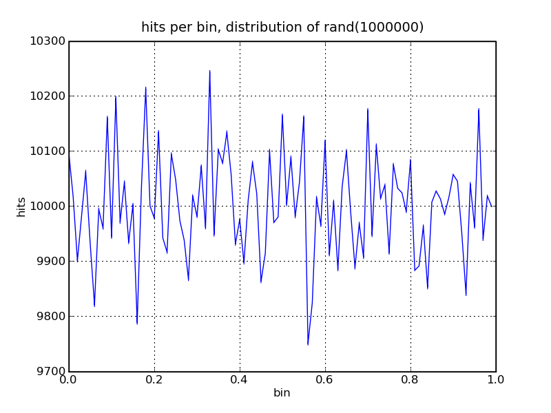 1,000,000 uniformly distributed samples
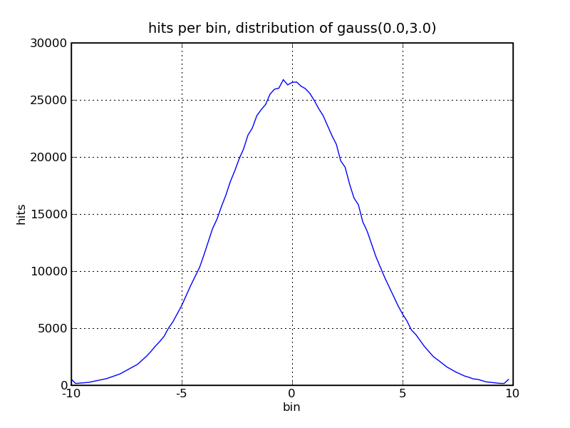 1,000,000 Gaussian distributed samples, mean=0.0, sigma=3.0
HW3 due by midnight of next class
1,000,000 Gaussian distributed samples, mean=0.0, sigma=3.0
HW3 due by midnight of next class
<- previous index next ->
-
CMSC 455 home page
-
Syllabus - class dates and subjects, homework dates, reading assignments
-
Homework assignments - the details
-
Projects -
-
Partial Lecture Notes, one per WEB page
-
Partial Lecture Notes, one big page for printing
-
Downloadable samples, source and executables
-
Some brief notes on Matlab
-
Some brief notes on Python
-
Some brief notes on Fortran 95
-
Some brief notes on Ada 95
-
An Ada math library (gnatmath95)
-
Finite difference approximations for derivatives
-
MATLAB examples, some ODE, some PDE
-
parallel threads examples
-
Reference pages on Taylor series, identities,
coordinate systems, differential operators
-
selected news related to numerical computation