<- previous index next ->
There may be times when you have to do numerical computation
on complex values (scalars, vectors, or matrices).
If you are programming in Fortran, no problem, the types
complex and complex*16 or double complex are built in.
In Ada 95, the full set of complex arithmetic and functions
come with the compiler as packages. MatLab and Python use
complex as needed, automatically (e.g. output of FFT).
In other programming languages you need to know how to do
complex computation and how to choose the appropriate
numerical method.
older
C Java Fortran 95 Fortran Ada 95 MATLAB Python
------ ------ ---------------- ---------- ------------ -------- --------
complex
32 bit 'none' 'none' complex complex complex N/A N/A
64 bit 'none' 'none' double complex complex*16 long_complex 'default' 'default'
'none' means not provided by the language (may be available as a library)
N/A means not available, you get the default.
Background:
A complex number is stored in the computer as an ordered pair
of floating point numbers, the real part and the imaginary part.
The floating point numbers may be single or double precision as
needed by the application. It is suggested that you use double
precision as the default.
These are called Cartesian coordinates. Polar coordinates are
seldom used for computation, yet, are usually made available by
a conversion function to magnitude and angle. Note that
numerical analyst call the angle by the name "argument".
The naming convention depends on the programming language and
personal (or customer) choice.
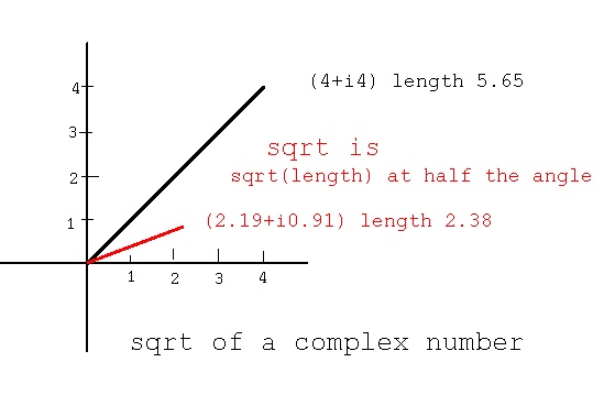
Basic complex arithmetic is covered first and then complex
functions: sin, cos, tan, sinh, cosh, tanh, exp, log, sqrt, pow
are covered in the next lecture.
The simplest need for complex numbers is solving for the roots
of the polynomial equation x^2 + 1 = 0 .
There must be exactly two roots and they are sqrt(-1) and
-sqrt(-1) that are named "i" and "-i".
The quadratic equation for finding roots of a second order
polynomial should use the complex sqrt, even for real coefficients
a, b, and c, because the roots may be complex.
given: a x^2 + b x + c = 0 find the roots
b +/- sqrt(b^2 - 4 a c)
solution x = -----------------------
2 a
that computes complex roots if 4 a c > b^2
Of course, the equation correctly computes the roots when
a, b, and c are complex numbers.
Complex Arithmetic
i=sqrt(-1) indicates imaginary part. a and b are real numbers.
(a+ib) is just two real numbers with b interpreted as imaginary.
Complex numbers are added by adding the real and imaginary parts:
(a+ib) + (c+id) = (a+c) + i(b+d)
Similarly, subtraction:
(a+ib) - (c+id) = (a-c) + i(b-d)
The multiplication of two complex numbers is:
(a+ib)*(c+id) = (a*c - b*d) + i(b*c + a*d)
The division of two complex numbers is:
r = c*c + d*d
(a+ib)/(c+id) = (a*c + b*d)/r + i(b*c - a*d)/r
Existing Implementations
The basic complex arithmetic (including some functions for
the next lecture) are in Complex.java
The automatically generated documentation is Complex.html
The complex arithmetic and functions in C uses "cx" named functions
as shown in the header file complex.h
and the body complex.c
with a test program test_complex.c
with results test_complex_c.out
The built in Ada package generic_complex_types.ads
provides complex arithmetic. Note the many operator definitions.
The use of complex in Ada is shown in this small program:
complx.adb
Complex functions are provided by generic_complex_elementary_functions.ads
The use of complex in Fortran 95 is shown in this small program:
complx.f90
C++ has the STL class Complex and can be used as shown
test_complex.cpp
test_complex_cpp.out
Python example
test_complex.py3
test_complex_py3.out
test_cxmath.py3
test_cxmath_py3.out
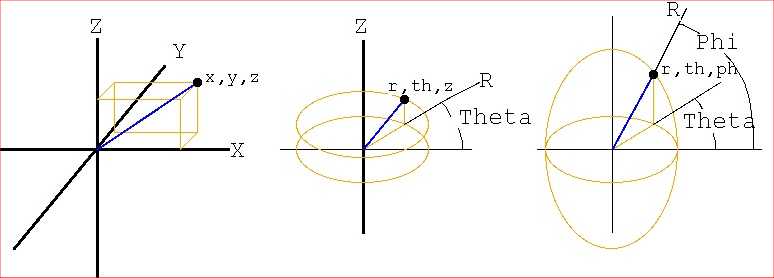
Cartesian Coordinates
Complex numbers define a plane and are typically Cartesian coordinates.
Polar coordinates also define a plane in terms of radius, r and angle θ.
x = r * cos(θ) r = sqrt(x*x+y*y)
y = r * sin(θ) θ = arctan(y/x) or atan2
Other coordinate systems are:
Cylindrical Coordinates
Cylindrical coordinates in terms of radius r, angle θ and height z.
x = r * cos(θ) r = sqrt(x*x+y*y)
y = r * sin(θ) θ = arctan(y/x) or atan2
z = z z = z
Spherical Coordinates
Spherical coordinates in terms of radius r, angles θ and φ
x = r * sin(φ) * cos(θ) r = sqrt(x*x+y*y+z*z)
y = r * sin(φ) * sin(θ) θ = arctan(y/x) or atan2
z = r * cos(φ) φ = arctan(sqrt(x*x+y*y)/z)
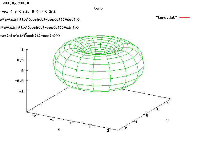
Toroidal Coordinates 1
The five independent variables are a, σ, θ, φ and z0
denom = cosh(θ)-cos(σ)
x = a * sinh(θ) * cos(φ) / denom
y = a * sinh(θ) * sin(φ) / denom
z = a * sin(σ) / denom optional + z0
-π < σ < π θ > 0 0 < φ < 2π a > 0
φ = arctan(y/x)
temporaries r1 = sqrt(x^2 + y^2)
d1 = sqrt((r1+a)^2 + z^2)
d2 = sqrt((r1-a)^2 + z^2)
θ = ln(d1/d2)
σ = arccos((d1^2+d2^2-4*a^2)/(2*d1*d2))
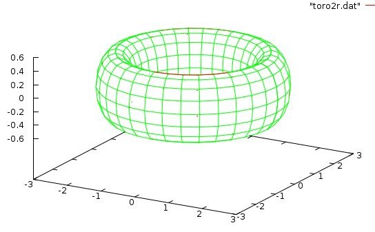
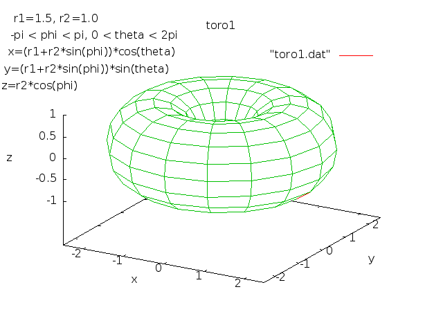
Toroidal Coordinates 2
The five independent variables are r1, r2, θ, φ, and z0
x = (r1 + r2 * sin(φ)) * cos(θ)
y = (r1 + r2 * sin(φ)) * sin(θ)
z = r2 * cos(φ) Optional + z0
0 < θ < 2π 0 < φ < 2π r1 > 0 r2 > 0
θ = arctan(y/x)
φ = arccos(z/r2)
r1 = x/cos(θ) - r2*sin(φ) or
r1 = y/sin(θ) - r2*sin(φ) no divide by zero
plot_toro.java try "run" etc
A simple implementation in C is demonstrated in
coordinate.c
coordinate.out
Beware of your choice of angle ranges when converting the above
radians to degrees.
 Cartesian Cylindrical Spherical
For Toroidal Coordinates 1:
toroidal_coord.c
toroidal_coord_c.out
toro.dat
toro.sh
toro.plot
Cartesian Cylindrical Spherical
For Toroidal Coordinates 1:
toroidal_coord.c
toroidal_coord_c.out
toro.dat
toro.sh
toro.plot
 For Toroidal Coordinates 2:
toro2r.c
toro2r_c.out
toro2r.dat
toro2r.sh
toro2r.plot
For Toroidal Coordinates 2:
toro2r.c
toro2r_c.out
toro2r.dat
toro2r.sh
toro2r.plot
 or
toroidal1_coord.c
toroidal1_coord_c.out
toro1.dat
toro1.sh
toro1.plot
or
toroidal1_coord.c
toroidal1_coord_c.out
toro1.dat
toro1.sh
toro1.plot
 Then, for later, differential operators in three coordinate systems
del and other operators
Del_in_cylindrical_and_spherical_coordinates
Fast accurate numerical computing of derivatives and partial derivatives
is covered in
CS455 lecture 24 Derivatives
CS455 lecture 24a Partial Derivatives
If you need angles between vectors in two, three, four dimensions:
angle_vectors.py3 source code
angle_vectors_py3.out
Then, for later, differential operators in three coordinate systems
del and other operators
Del_in_cylindrical_and_spherical_coordinates
Fast accurate numerical computing of derivatives and partial derivatives
is covered in
CS455 lecture 24 Derivatives
CS455 lecture 24a Partial Derivatives
If you need angles between vectors in two, three, four dimensions:
angle_vectors.py3 source code
angle_vectors_py3.out
<- previous index next ->
-
CMSC 455 home page
-
Syllabus - class dates and subjects, homework dates, reading assignments
-
Homework assignments - the details
-
Projects -
-
Partial Lecture Notes, one per WEB page
-
Partial Lecture Notes, one big page for printing
-
Downloadable samples, source and executables
-
Some brief notes on Matlab
-
Some brief notes on Python
-
Some brief notes on Fortran 95
-
Some brief notes on Ada 95
-
An Ada math library (gnatmath95)
-
Finite difference approximations for derivatives
-
MATLAB examples, some ODE, some PDE
-
parallel threads examples
-
Reference pages on Taylor series, identities,
coordinate systems, differential operators
-
selected news related to numerical computation